Mathematics 216 Computer-oriented Approach to Statistics
Self-Test B (Computer Component) Solutions
Self-Test 1B Solutions
Each Guided Solution below summarizes key Quick Reviews (QR) steps—but not all steps—needed to complete the problem in Self‑Test1B. These QRs will be useful when you are preparing for the computer components of the assignments, midterm exam, and final exam. For more detailed steps, see the relevant Computer Lab and Activity.
QRs are in italics; steps are separated by arrows →.
Problem 1. Create a data file and a solutions file.
1a. Create a StatCrunch data file called TastyExpress. Input the 25 customer responses to the TastyExpress survey (based on Figure 2).
Guided Solution 1a
Computer Lab 1A, Activity 2.Open the StatCrunch software from within the StatCrunch website.
www.StatCrunch.com → Sign in → Open StatCrunch
Computer Lab 1A, Activity 3.Collect data with a survey; enter and save the data in StatCrunch; and sign out of StatCrunch.
Open StatCrunch → Enter variable names in data file → Enter data values in data file → Data → Save → File Name: TastyExpress → Delimiter: space → Save → StatCrunch → Sign out
Computer Lab 1A, Activity 4.Open a data file that you have saved in your My Data folder on the StatCrunch website.
www.StatCrunch.com → Sign in → My StatCrunch → My Data → TastyExpress
Computer Lab 1A, Activity 6.Export data from a StatCrunch data file to a spreadsheet file.
With data displayed in a StatCrunch data file → Data → Export → Select all variables → File name → Delimiter: comma
Computer Lab 1A, Activity 7.Copy and paste data from a spreadsheet file to a Word file.
With data displayed in the spreadsheet → Select all variables and data in the spreadsheet (Ctrl+A) → Copy the selected variables and data (Ctrl+C) → Open the Word file → Paste the selected variables and data into the Word file (Ctrl+V)
Data file:
| Gender | Satisfy | Child | Coupon | Spend | Visits | Income | Age |
| 1 | 1 | 1 | 1 | 130 | 14 | 4000 | 29 |
| 1 | 1 | 1 | 1 | 195 | 15 | 4500 | 25 |
| 2 | 3 | 2 | 3 | 12 | 4 | 6250 | 44 |
| 1 | 2 | 1 | 1 | 260 | 14 | 3100 | 30 |
| 2 | 2 | 2 | 3 | 23 | 6 | 5250 | 37 |
| 1 | 1 | 1 | 1 | 175 | 12 | 4250 | 32 |
| 2 | 2 | 2 | 2 | 25 | 7 | 7000 | 41 |
| 1 | 1 | 1 | 2 | 180 | 13 | 4300 | 28 |
| 1 | 1 | 1 | 1 | 170 | 15 | 6100 | 26 |
| 2 | 3 | 1 | 3 | 15 | 7 | 7200 | 43 |
| 2 | 3 | 2 | 3 | 16 | 6 | 6900 | 46 |
| 1 | 1 | 1 | 1 | 185 | 15 | 5200 | 29 |
| 2 | 3 | 1 | 3 | 23 | 7 | 6800 | 44 |
| 1 | 1 | 1 | 2 | 215 | 13 | 5000 | 32 |
| 1 | 2 | 1 | 1 | 155 | 12 | 4400 | 30 |
| 2 | 3 | 2 | 3 | 12 | 5 | 6500 | 42 |
| 2 | 2 | 2 | 3 | 19 | 6 | 7700 | 41 |
| 1 | 1 | 1 | 1 | 225 | 16 | 5000 | 23 |
| 1 | 1 | 2 | 1 | 215 | 18 | 5400 | 26 |
| 1 | 2 | 1 | 1 | 149 | 12 | 5300 | 24 |
| 2 | 3 | 2 | 3 | 9 | 4 | 7350 | 42 |
| 1 | 2 | 1 | 1 | 255 | 13 | 4900 | 25 |
| 2 | 3 | 2 | 3 | 200 | 14 | 10500 | 40 |
| 2 | 3 | 2 | 3 | 15 | 5 | 7300 | 39 |
| 1 | 1 | 1 | 1 | 245 | 12 | 5300 | 23 |
1b. Export all the quantitative variables along with the first five data values for each quantitative variable from the StatCrunch file to a csv comma delimited file (spreadsheet file).
Guided Solution 1b
Computer Lab 1A, Activity 4.Open a data file that you have saved in your My Data folder on the StatCrunch website.
www.StatCrunch.com → Sign in → My StatCrunch → My Data → TastyExpress
Computer Lab 1A, Activity 6.Export data from a StatCrunch data file to a spreadsheet file.
With data displayed in the StatCrunch data file: Data → Export → Select quantitative variables → File name → Delimiter: comma
Computer Lab 1A, Activity 7.Copy and paste data from a spreadsheet file to a Word file.
With data displayed in the spreadsheet → Select the quantitative variables and related five data values in the spreadsheet → Copy the selected variables and data (Ctrl C) → Open the Word file → Paste the selected variables and data into the Word file (Ctrl V)
First five data values for the quantitative STAT101 survey variables pasted from a spreadsheet to a Word file:
| Spend | Visits | Income | Age |
| 130 | 14 | 4000 | 29 |
| 195 | 15 | 4500 | 25 |
| 12 | 4 | 6250 | 44 |
| 260 | 14 | 3100 | 30 |
| 23 | 6 | 5250 | 37 |
Problem 2. Recode variables to text descriptions and export them to a spreadsheet file.
Guided Solution 2
Computer Lab 1A, Activity 4.Open the TasyExpress data file that you have saved in your My Data folder on the StatCrunch website.
www.StatCrunch.com → Sign in → My StatCrunch → My Data → TastyExpress
Computer Lab 1B, first part of Activity 5.Recode qualitative variable.s
Computer Lab 1A, Activity 6.Export data from a StatCrunch data file to a spreadsheet file.
With data displayed in a StatCrunch data file → Data → Export → Select recoded variables → File Name → Delimiter: comma
Computer Lab 1A, Activity 7.Copy and paste data from a spreadsheet file to a word file.
With data displayed in the spreadsheet → Select the recoded variables and related five data values in the spreadsheet → Copy the selected variables and data (Ctrl C) → Open the Word file → Paste the selected variables and data into the Word file (Ctrl V) → Save the updated Word file.
Save the recoded StatCrunch data file under the file name TastyExpress Recoded.
Data → Save → File Name: TastyExpress Recoded → Delimiter: space → Save
First 5 recoded variables pasted to Word file:
| Recode(Gender) | Recode(Satisfy) | Recode(Child) | Recode(Coupon) |
| Female | VSat | Yes | Freq |
| Female | VSat | Yes | Freq |
| Male | LSat | No | Never |
| Female | Sat | Yes | Freq |
| Male | Sat | No | Never |
Problem 3. Create and interpret a pie chart.
3a. Construct a pie chart for the Gender variable: Relative Frequency.
Guided Solution 3a
Computer Lab 1B, Activity 5. Construct a pie chart to analyze qualitative survey data.
Graph → Pie Chart → With data → Recode(Gender) → Percent of Total
Computer Lab 1B, second part of Activity 5.Copy the pie chart into your Word file.
Click Options on the graph window → Copy → Right-click on the graph window → Copy image → Click in the Word file → Paste Special → Device Independent Bitmap
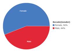
Pie chart pasted into word processing file.
3b. Females are the most frequent gender category surveyed (56% vs. 44%).
Problem 4. Determine and interpret modes of qualitative variables.
4a. Display the mode for the variables Satisfy, Child, and Coupon.
Guided Solution 4a
Computer Lab 1A, Activity 8.Work with measures of central tendency: mean, median, mode.
Stat → Summary Stats → Columns → Select variables → Select Mode
Computer Lab 1A, second part of Activity 8.
With the StatCrunch summary statistics table displayed → Click in Summary Statistics table →
Ctrl A → Ctrl C → With the Word file displayed and your cursor under Problem 4a subheading → Ctrl V
Pasted summary statistics table:
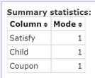
4b. Type the mode for variables Satisfy, Child, and Coupon, and interpret the results in terms of the appropriate recoded values.
- Mode for Satisfy is 1 or VSat, meaning the most frequent response is very satisfied.
- Mode for Child is 1 or Yes, meaning the most frequent response is bring children.
- Mode for Coupon is 1 or Frequently, meaning the most frequent response is frequently use coupons.
Problem 5. Create and interpret a Pareto chart.
5a. Construct a Pareto chart for the Recode(Satisfy) variable.
Guided Solution 5a
Computer Lab 1B, Activity 6. Construct a Pareto chart for qualitative data.
Graph → Bar Plot → With Data → Select Column variable → Select Frequency as Type → Count Descending Order → Display Value above bar
Computer Lab 1B, second part of Activity 6.Paste the Pareto chart into a Word file.
Click Options on the graph window → Copy → Right-click on the graph window → Copy Image → Click in the Word file → Paste Special → Device Independent Bitmap
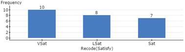
Pareto chart pasted into word processing file.
5b. The Pareto chart indicates a relatively high level of consumer satisfaction, with the categories very satisfied and satisfied making up 17 of the 25 responses.
Problem 6. Create and interpret a frequency table.
6a. Construct a frequency table for Age, using 6 bins with a starting value of 20 and a fixed bin width of 5.
The frequency table should have 6 bins(classes) with a starting value of 20 and a fixed bin width of 5 where each bin includes the left endpoint. The frequency table should display: Frequencies, Relative Frequencies, and Cumulative Relative Frequencies. Copy and paste the frequency table to your Word file.
Guided Solution 6a
Computer Lab 1B, Activity 1.Construct a frequency distribution with classes.
Create a bins column: Data → Bin → Select Column → Define Bins: Use Fixed Width bins, Start-at Value, Bin-width Value → Bin Edges: Include Left Endpoint
Create a frequency table: Stat → Tables → Frequency → Select Bin Column →
Use Ctrl key to select multiple statistics: Frequency, Relative Frequency, Cumulative Relative Frequency etc... → Order by Value Ascending
Computer Lab 1B, second part of Activity 1.Copy and paste the frequency table into a Word file.
With the StatCrunch frequency table displayed → Click in the table → Ctrl A → Ctrl C → With the Word file open and your cursor under Problem 6a subheading → Ctrl V
Frequency table results for Bin(Age). Count = 25
| Bin(Age) | Frequency | Relative Frequency | Cumulative Relative Frequency |
| 20 to 25 | 3 | 0.12 | 0.12 |
| 25 to 30 | 7 | 0.28 | 0.4 |
| 30 to 35 | 4 | 0.16 | 0.56 |
| 35 to 40 | 2 | 0.08 | 0.64 |
| 40 to 45 | 8 | 0.32 | 0.96 |
| 45 to 50 | 1 | 0.04 | 1 |
6b. The 40–45 age category is the most frequent class.
6c. 28% of those surveyed were between 25 to 30 years of age.
6d. 56% of those surveyed were under 35 years of age.
Problem 7. Create and interpret a histogram.
7a. Construct a histogram for Visits using 4 bins with a starting value of 0 and a fixed bin width of 5.
The frequency table should display: Relative Frequencies. Copy and paste the histogram to your Word file.
Guided Solution 7a
Computer Lab 1B, Activity 2.Construct a frequency histogram.
Graph → Histogram → Select Column: Visits → Select Type: Relative Frequency → Define Bins →
Copy and paste the graph into a word file:
With the frequency histogram window displayed in StatCrunch, click Options on the graph window → Copy → Right-click on the graph window → Copy Image → Click in the Word file → Paste Special → Device Independent Bitmap
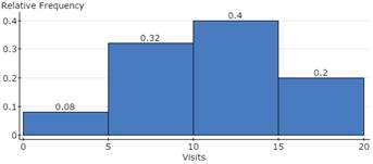
7b. The 10–15 visits per month category is the most frequent class.
7c. 40% of those surveyed visit TastyExpress between 10 and 15 times per month.
Problem 8. Analyze the variable Visits.
8a. Use StatCrunch to determine the mean, median, standard deviation, variance, first quartile, median, third quartile, and interquartile range for the variable Visits in the TastyExpress survey.
Copy and paste the Summary Statistics Table displaying all these statistics to your Word file.
Guided Solution 8a
Computer Lab 1B, Activities 8, 9, 10.Measures of Central Tendency, Variation, and Position.
Stat → Summary Stats → Columns → Select Columns: Visits → Select Statistics: Mean, Median, Std. dev., Q1, Q3, IQR
Computer Lab 1B, second part of Activity 1.Copy and paste the table into a Word file.
With the StatCrunch Summary Statistics table displayed → Click in the table → Ctrl A → Ctrl C → With the Word file open and your cursor under Problem 8a subheading → Ctrl V
Pasted summary statistics table:
Summary statistics
| Column | Mean | Std. dev. | Median | Q1 | Q3 | IQR |
| Visits | 10.6 | 4.3493295 | 12 | 6 | 14 | 8 |
8b. 75% of the customers visited TastyExpress more than 6 times per month (Q1).
Problem 9. Analyze the monthly visits.
9a. Use StatCrunch to compute the mean and standard deviation monthly visits for each of the Gender subsets: male and female customers.
Copy and paste the Summary Statistics table displaying these statistics to your Word file.
Guided Solution 9a
Computer Lab 1B, Activity 12. Apply tools of descriptive statistics to subsets of data.
Stat → Summary Stats → Columns → Select Columns: Visits → Select Statistics: Mean, Std. dev. → Select variable to group by: Recode(Gender)
Computer Lab 1B, second part of Activity 1.Copy and paste the table into a Word file.
With the StatCrunch Summary Statistics table displayed → Click in the table → Ctrl A → Ctrl C → With the Word file displayed and your cursor under Problem 9a subheading → Click Ctrl V
Pasted Summary Statistics Table: Mean and standard deviation, Visits by Gender:
Summary statistics for Visits. Group by: Recode(Gender)
| Recode(Gender) | Mean | Std. Dev. |
| Female | 13.857143 | 1.7913099 |
| Male | 6.4545455 | 2.733629 |
9b. Under the subheading 9b, type:
The number of monthly visits made by female customers (13.85714) significantly exceeds the number of monthly visits made by male customers (6.4545).
Problem 10. Analyze the monthly amount spent.
10a. Use StatCrunch to compute the mean and standard deviation monthly amount spent for each of the Gender subsets: male and female customers.
Copy and paste the Summary Statistics table displaying these statistics to your Word file.
Guided Solution 10a
Computer Lab 1B, Activity 12. Apply tools of descriptive statistics to subsets of data.
Stat → Summary Stats → Columns → Select Columns: Spend → Select Statistics: Mean, Std. dev. → Select variable to group by: Recode(Gender)
Computer Lab 1B, second part of Activity 1.Copy and paste the table to your Word file.
With the StatCrunch Summary Statistics table displayed → Click in the table → Ctrl A → Ctrl C
With the Word file displayed and your cursor under Problem 9a subheading → Click Ctrl V
Pasted Summary Statistics Table: Mean and Standard Deviation Spent By Gender:
Summary statistics for Spend. Group by: Recode(Gender).
| Gender | Mean | Std. dev. |
| Female | 196.71429 | 40.454017 |
| Male | 33.545455 | 55.444321 |
10b. Under the subheading 10b, type:
The monthly amount spent by female customers ($196.71429) significantly exceeds the number of monthly visits made by male customers ($33.545455).
Problem 11. Create and interpret box-and-whisker plots.
11a. Use StatCrunch to create two box-and-whisker plots.
The plots must compare the monthly number of visits made by customers who frequently bring children to TastyExpress with the monthly number of visits made by customers who do NOT frequently bring children to TastyExpress. Copy and paste the box-and-whisker plots to your Word file.
Guided Solution 11a
Computer Lab 1B, Activity 11.Construct a box-and-whisker plot for quantitative data.
Graph → boxplot → Select Columns: Visits → Group By: Recode(Child) → Draw boxes horizontally
Computer Lab 1B, second part of Activity 2.Copy and paste the graph into a Word file.
With the graph window displayed in StatCrunch → Click Options on the graph window → Copy → Right-click on the graph window → Copy Image → Click in the Word file → Paste Special → Device Independent Bitmap
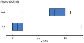
Pasted box-and-whisker plots for visits by child subsets.
11b. If you move your cursor over each box plot in StatCrunch, you will see that the median monthly visits for customers who frequently bring children is 13, while the median monthly visits for customers who do NOT frequently bring children is 6.
Problem 12. Create and interpret a contingency table.
12a. Use StatCrunch to create a contingency table.
The contingency table must examine the relationship between the two variables Recode(Gender) and Recode(Satisfy). Select Recode(Gender) as the row variable and Recode(Satisfy) as the column variable. Display the Row percentage in the table.
Guided Solution 12a
Computer Lab 1B, Activity 13.Contingency table analysis: Relationship between two survey variables.
Stat → Tables → Contingency → With data → Select Row variable, Column variable → Select Row percent → Copy and paste the table into the Word file SelfTest1B, under the subheading Problem 12a.
With the StatCrunch Contingency table displayed → Click in the table → Ctrl A → Ctrl C → With the Word file displayed and your cursor under Problem 12a subheading → Ctrl V
Pasted Contingency Table:
Contingency table results:
Rows: Recode(Gender)
Columns: Recode(Satisfy)
| Cell format |
| Count (Row %) |
| LSat | Sat | VSat | Total | |
| Female | 0 (0%) |
4 (28.57%) |
10 (71.43%) |
14 (100%) |
| Male | 8 (72.73%) |
3 (27.27%) |
0 (0%) |
11 (100%) |
| Total | 8 (32%) |
7 (28%) |
10 (40%) |
25 (100%) |
12b. While 71.43% of the female customers are very satisfied with TastyExpress, 0% of the males are very satisfied with TastyExpress. Put differently, 72.73% of the males are less than satisfied with Tasty Express.
Problem 13. Simulate coin tossing.
13a. Generate random integers so as to simulate tossing a coin 200 times.
Let 1 represent heads, and 2 represent tails. Allow repeats. Copy and paste all the numbers generated in the StatCrunch Random Number window to the first variable column in the blank StatCrunch data file, with the first pasted value located in Row 1. Type Coin as the name of this first variable.
Recode the 1 to show as Heads and the 2 to show as Tails and store the results in the second column, with the variable name displayed as Recode(Coin).
Create a frequency table for the variable Recode(Coin), which displays the frequency and relative frequency.
Copy and paste the frequency table from StatCrunch to the Word file SelfTest1B, under the subheading Problem 13a.
Guided Solution 13a
Computer Lab 1A, Activity 8.Technology exercises for random numbers.
Open StatCrunch → Applets → Random numbers → Once the 200 random numbers display in the Random number window, hold down the left mouse button and scroll down to select all 200 numbers → Press Ctrl C to copy the numbers → Click in row 1 of the first variable column in the data file → Press Ctrl V to paste all 200 numbers into the first 200 rows of the first column in the data file → Type Coin as the column name.
Computer Lab 1B, first part of Activity 5.
Data → Recode → Coin → Compute → Heads, Tail
Computer Lab 1B, second part of Activity 1.Construct a frequency distribution (no bins required here).
Stat → Tables → Frequency → Select Recode(Coin) → Use Ctrl key to select multiple statistics: Frequency, Relative frequency,... → Order by Value Ascending
Computer Lab 1B, third part of Activity 1.Copy and paste a table into a Word file.
With the Frequency Table window displayed in StatCrunch, copy and paste the table into the Word file SelfTest1B, under the subheading Problem 13a.
Click Options on the frequency table window → Copy → Click on the frequency table window → Ctrl A → Ctrl C → Click in the Word file under Problem 12a → Ctrl V
Pasted frequency table for simulated coin toss:
Frequency table results for Recode(Coin).
Count = 200
| Recode(Coin) | Frequency | Relative Frequency |
| Tails | 94 | 0.47 |
| Heads | 106 | 0.53 |
13b. Theoretically, you would expect to see the relative frequency of the Heads category to be close to 0.50 or 50%. Because random integers are used, solutions will vary.
Self-Test 2B Solutions
Each Guided Solution below summarizes key Quick Reviews (QR) steps—but not all steps—needed to complete the problem in Self‑Test2B. These QRs will be useful when you are preparing for the computer components of the assignments, midterm exam, and final exam. For more detailed steps, see the relevant Computer Lab and Activity.
QRs are in italics; steps are separated by arrows →.
Problem 1. Work with random numbers and probability.
1a. Use StatCrunch to generate random numbers between 1 and 6, to simulate the tossing of one die 500 times.
Create the StatCrunch data file OneDie, showing the results of the simulation of 500 repetitions of a toss of one die. Copy and paste the variable name and the first 5 die numbers that were observed from StatCrunch to a Word file called SelfTest2B.
The results will differ for each student. The results observed by the course author are shown below:
| Die |
| 6 |
| 5 |
| 2 |
| 5 |
| 3 |
Guided Solution 1a
Computer Lab 1, Activity 2.Open the StatCrunch Software from within the StatCrunch website.
www.StatCrunch.com → Sign in → Open StatCrunch
Computer Lab 2, Activity 3.Simulate the outcomes of the game of chance using random numbers:
Applets → Random Numbers → Type Minimum Value → Type Maximum Value → Type Sample Size → Allow Repeats → Compute
Computer Lab 2, Activity 3.Copy and paste random numbers to column in data file:
Select all random numbers generated in options window → Ctrl C → Click in first row of data file columns → Ctrl V
Computer Lab 1, Activity 7.Copy and paste data from a StatCrunch data file to Word file:
With data displayed in a StatCrunch data file:
Select the variable name and related five data values in the data file → Copy the selected variable and data (Ctrl C) → Open a Word file → Paste the selected variable and data into the Word file (Ctrl V) → Save the updated file.
1b. Referring to Problem 1a above, consider this event: The die number that comes up will be at least 3. This number could be 3, 4, 5, or 6.
In the StatCrunch data file OneDie, create the recoded variable Recode(Die) with two values: “At Least 3” and “Less Than 3”. Use StatCrunch to compute the approximate probability of the event “At Least 3” by creating a frequency table for the variable Recode(Die).
Copy and paste the two variable names, Die and Recode(Die), and the first five values for each of these variables from StatCrunch to the Word file SelfTest2B under the subheading Problem 1b.
Copy and paste the frequency table you created from StatCrunch to the Word file SelfTest2B under the subheading Problem 1b.
The results that the course author obtained are below:
| Die | Recode(Die) |
| 6 | At Least 3 |
| 5 | At Least 3 |
| 2 | Less Than 3 |
| 5 | At Least 3 |
| 3 | At Least 3 |
Based on the frequency table created by the course author (below), the Probability (At Least 3) = 0.706
Frequency table results for Recode(Die):
Count = 500
| Recode(Die) | Frequency | Relative Frequency |
| At Least 3 | 353 | 0.706 |
| Less Than 3 | 147 | 0.294 |
Guided Solution 1b
Computer Lab 2, Activity 3.Recode the random numbers pasted to the data file:
Data → Recode → Select column variable → Compute → Recode each numerical value to text-based description
Computer Lab 2, Activity 3.Create a relative frequency table:
Stat → Tables → Frequency → Select Recode variable → Select Relative Frequency → Compute
Computer Lab 1B, second part of Activity 1.Paste a table into a Word file:
With the StatCrunch frequency table displayed → Click in table → Ctrl A → Ctrl C → With the Word file displayed and your mouse pointer under Problem 1b subheading → Ctrl V
1c. Theoretically (based on the classical view of probability), you should expect to see the relative frequency of the “At Least 3” category to be close to ____?
Solution 1c
Theoretically, you should expect to see the relative frequency of the “At Least 3” category to be close to (4 outcomes/6 possible outcomes) = 0.67.
Problem 2. Probability and random numbers
2a. Consider the following probability experiment:
A pair of dice is tossed and you are interested in observing the totalof the two numbers that come up on the dice. For example, if a pair of ones (1,1) appears, the total is 2. If the two dice show a 5 on the first die and 3 on the second die (5,3) the total is 8.
Create a StatCrunch data file called TwoDice, which contains the results from simulating 1,000 repetitions of a toss of two dice and observing the total of each set of two numbers.
Copy and paste the 3 variable names and the first 5 rows of the three Columns Die1, Die2, and Die1+Die2 from StatCrunch to the Word file SelfTest2B under the subheading Problem 2a. the results will differ for each student.
The results observed by the course author are below.
| Die1 | Die2 | Die1+Die2 |
| 1 | 6 | 7 |
| 2 | 5 | 7 |
| 4 | 1 | 5 |
| 3 | 2 | 5 |
| 5 | 2 | 7 |
Guided Solution 2a
Computer Lab 1, Activity 2.Open StatCrunch through the StatCrunch website:
www.StatCrunch.com → Sign on → Open StatCrunch
Computer Lab 2, Activity 3.Simulate the outcomes of the game of chance using random numbers:
Applets → Random numbers → Type minimum value → Type maximum value → Type sample size → Allow repeats → Click compute
Computer Lab 2, Activity 3.Copy and paste random numbers to column in data file:
Select all random numbers generated in options window → Ctrl C → Click In first row of data file columns → Ctrl V
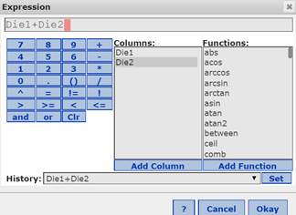
New Activity: Create a new column variable by calculating row totals of existing variables:
With the 1000 random values displayed in each of the two variable Columns Die1 and Die2: Data → Compute → Expression → In the Compute Expression box, click Build to display the Expression box → In the Columns section, click Die1 → click Add Column → Click the + sign on the virtual calculator keyboard → In the Columns section, click Die2 → click the Add Column button (see figure below) → Click Okay, then click Compute, to create the third variable column Die1+Die2
Computer Lab 2, second part of Activity 1:Copy and paste data from a StatCrunch data file to Word file:
With data displayed in a StatCrunch data file → Select the three variable names and related five data values in the data file → Copy the selected variables and data (Ctrl C) → Open a Word file → Paste the selected variables and data into the Word file (Ctrl V) → Save the updated document.
2b. Refer to the probability experiment in Problem 2a, in which a pair of dice is tossed and the total of the two numbers that appear is observed. Consider the event “the dice total will be at least 10.” This means that the dice total could be 10, 11, or 12.
In the StatCrunch data file TwoDice, create the recoded variable Recode(Die1+Die2) with two value: “At Least 10” and “Less Than 10”. Use StatCrunch to compute the approximate probability of the event “At Least 10” by creating a frequency table for the variable Recode(Die1+Die2).
Copy and paste the four variable names, Die1, Die2, Die1+Die2, and Recode(Die1+Die2), with the first five values for each of these variables, from StatCrunch to the Word file SelfTest2B under the subheading Problem 2a.
Copy and paste the frequency table that you created from StatCrunch to the Word file SelfTest2B under the subheading Problem 2b.
The results the course author obtained are shown below. Based on the frequency table, the Probability (At Least 10) = 0.191.
| Die1 | Die2 | Die1+Die2 | Recode(Die1+Die2) |
| 6 | 3 | 9 | Less than 10 |
| 4 | 1 | 5 | Less than 10 |
| 4 | 2 | 6 | Less than 10 |
| 4 | 2 | 6 | Less than 10 |
| 6 | 5 | 11 | At Least 10 |
Frequency table results for Recode(Die1+Die2):
Count = 1000
| Recode(Die1+Die2) | Frequency | Relative Frequency |
| At Least 10 | 191 | 0.191 |
| Less Than 10 | 809 | 0.809 |
Guided Solution 2b
Computer Lab 2, Activity 3.Recode the random numbers pasted to the data file:
Data → Recode → Select column variable → Compute → Recode each numerical value to text-based description →
Computer Lab 2, Activity 3.Create a relative frequency table:
Stat → Tables → Frequency → Select Recode variable → Select Relative Frequency → Compute
2c. Theoretically (based on the classical view of probability), you should expect to see the relative frequency of the “At Least 10” category to be close to ____?
Solution 2c
Theoretically (based on the classical view of probability), you should expect to see the relative frequency of the “At Least 10” category to be close to 6/36 = 0.17. This is based on the observation that there are 6 (out of 36) different possible outcomes that can occur for the event “At Least 10” to occur: ((4,6), (6,4), (5,5), (5,6), (6,5), (6,6))
Problem 3. Relative frequency of an event
3a. In the StatCrunch data file TwoDice, create a second recoded variable Recode(Die1+Die2) with two values.
In the StatCrunch data file TwoDice, create a second recoded variable Recode(Die1+Die2) with two values: “At Most 5” and “More than 5”. Use StatCrunch to compute the approximate probability of the event “At Most 5” by creating a frequency table for the second recoded variable Recode(Die1+Die2). Copy and paste the frequency table you created from StatCrunch to the Word file SelfTest2B under the subheading Problem 3a.
Based on the frequency table created by the course author (below), the Probability (At Most 5) = 0.282.
Frequency table results for Recode(Die1+Die2):
Count = 1000
| Recode(Die1+Die2) | Frequency | Relative Frequency |
| At Most 5 | 282 | 0.282 |
| More Than 5 | 718 | 0.718 |
Use StatCrunch to create a frequency table for the second recoded variable Recode(Die1+Die2) that displays the relative frequency for the two values “At Most 5” and “More Than 5”.
Guided Solution 3a
Computer Lab 2, Activity 3.Recode the dice totals as “At Most 5” and “More than 5”:
Data → Recode → Select Column variable → Compute → Recode each numerical value to text-based description
Computer Lab 2, Activity 3.Create a relative frequency table for recoded variable:
Stat → Tables → Frequency → Select Recode variable → Select Relative Frequency → Compute
3b. Theoretically (based on the classical view of probability) you should expect to see the relative frequency of the “At Most 5” category to be close to ____?
Solution 3b
Theoretically (based on the classical view of probability), you should expect to see the relative frequency of the “At Most 5” category to be close to 10/36 = 0.2777. This is based on the observation that there are ten (out of 36) different possible outcomes that can occur for the event “At Most 5” to occur: ((1,1), (2,1), (1,2), (1,3), (3,1), (2,2), (2,3), (3,2) (4,1), (1,4))
Problem 4. Sun Exposure survey
4a. Recode the responses.
Open the StatCrunch data-set file SunEx1 which is in the StatCrunch Groups folder AU Math216 2020.
With the StatCrunch SunEx1 data file displayed, create two recoded variables: Recode(Melanoma) and Recode(SkinColour).
Copy and paste the two recoded variables Recode(Melanoma) and Recode(SkinColour) and the first five values for each of these variables from StatCrunch to the Word file SelfTest2B under the subheading Problem 4a.
The results are shown below:
| Recode(Melanoma) | Recode(SkinColour) |
| 3-NeverDiag | 2-Medium |
| 3-NeverDiag | 1-Light |
| 3-NeverDiag | 1-Light |
| 3-NeverDiag | 2-Medium |
| 3-NeverDiag | 2-Medium |
Guided Solution 4a
Computer Lab 2, Activity 3.Recode variables Melanoma and SkinColour.
Data → Recode → Select column variable → Compute → Recode each numerical value to text-based description
4b. Use StatCrunch to construct a contingency table consisting of the two recoded variables Recode(Melanoma) and Recode(SkinColour).
Use StatCrunch to construct a contingency table consisting of the two recoded variables Recode(Melanoma) and Recode(SkinColour). Select Recode(Melanoma) as the row variable and Recode(SkinColour) as the column variable. Display both the Counts and Row Percents.
Copy and paste the contingency table to the Word file SelfTest2B under the subheading Problem 4b.
The results are shown below:
Contingency table results:
Rows: Recode(Melanoma)
Columns: Recode(SkinColour)
| Cell format |
| Count (Row percent) |
| 1-Light | 2-Medium | 3-Dark | 4-DoNotKnow | Total | |
| 1-Yes | 26 (61.9%) |
13 (30.95%) |
3 (7.14%) |
0 (0%) |
42 (100%) |
| 2-No | 62 (60.19%) |
36 (34.95%) |
5 (4.85%) |
0 (0%) |
103 (100%) |
| 3-NeverDiag | 1548 (40.2%) |
1841 (47.81%) |
459 (11.92%) |
3 (0.08%) |
3851 (100%) |
| 4-DoNotKnow | 7 (36.84%) |
10 (52.63%) |
2 (10.53%) |
0 (0%) |
19 (100%) |
| 5-NotStated | 4 (57.14%) |
2 (28.57%) |
0 (0%) |
1 (14.29%) |
7 (100%) |
| Total | 1647 (40.95%) |
1902 (47.29%) |
469 (11.66%) |
4 (0.1%) |
4022 (100%) |
Chi-Square test:
| Statistic | DF | Value | P‑value |
| Chi-square | 12 | 169.2917 | < 0.0001 |
Guided Solution 4b
Computer Lab 2, Activity 2, Empirical Probability.Computing probabilities involving multiple variables:
Create the appropriate contingency table.
Stat → Tables → Contingency → With Data → Select row variable → Select column variable → Display Row Percent → Compute
4c. Based on the contingency table you created, use your calculator (not StatCrunch) to compute the probability that a randomly selected adult Canadian responding to the survey will:
Solution 4c
- have Light skin colour = 1647/4022 = 0.4095
- have been diagnosed with malignant melanoma = 42/4022 = 0.0104
- have medium skin colour OR will be diagnosed with malignant melanoma = (1902 + 42-13)/4022 = 0.4801.
- have dark skin colour AND will be diagnosed with malignant melanoma = 3/4022 = 0.0007.
- have light colour skin, GIVEN that have been diagnosed with malignant melanoma = 26/42 = 0.6190
- determine, by making the appropriate math calculations, if the events “light skin colour” and “have been diagnosed with malignant melanoma” are independent events.
- P(light skin colour) = 1647/4022 = 0.4095
- P(light skin colour/have melanoma) = 26/42 = 0.6190
- Not Independent. Having melanoma is significantly increased where the person has light skin colour.
Self-Test 3B Solutions
Each Guided Solution below summarizes key Quick Reviews (QR) steps—but not all steps—needed to complete the problem in Self‑Test3B. These QRs will be useful when you are preparing for the computer components of the assignments, midterm exam, and final exam. For more detailed steps, see the relevant Computer Lab and Activity.
QRs are in italics; steps are separated by arrows →.
Problem 1. Dozens Bet in roulette
1a. Create the data file DozensBet, and the Word file Self Test3B.
Create a StatCrunch data file called DozensBet, which contains the probability distribution of the Dozens Bet in a roulette game. Copy and paste the probability to a Word file SelfTest3B.
The pasted table is displayed below.
| NetPayoff | P(X) |
| 2 | 0.3158 |
| −1 | 0.6842 |
Guided Solution 1a
Computer Lab 1A, Activity 2.Open StatCrunch through Pearson MyLab.
www.StatCrunch.com → Sign in → Open StatCrunch
Create the variables and enter the values that describe the population distribution:
Type NetPayoff as the first column variable → Enter the two values of NetPayoff → Type P(X) as the second column variable → Enter the two values of P(X)
Copy and paste the probability distribution table to the Word file:
Select the probability distribution table → Ctrl C → Ctrl V to paste to the Word file.
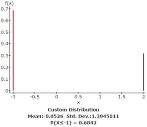
1b. Use StatCrunch to compute the mean and standard deviation of the probability distribution related to the Dozens Bet.
Use StatCrunch to compute the mean and standard deviation for the DozensBet probability distribution. Copy and paste the graph, mean and standard deviation of the probability distribution from StatCrunch to the Word file SelfTest3B under subheading Problem 1b. Your results should look the figure below.
Guided Solution 1b
Computer Lab 3A, Activity 1.Find the mean and standard deviation of a discrete random variable.
With the NetPayoff and P(X) column variables displayed in the data file:
Stat → Calculators → Custom → Select column variable X → Select column variable P(X) → Compute
To copy and paste the probability distribution graph to a Word file:
Click Options Copy → Click right mouse button in StatCrunch graph window → Copy Image → Paste Special → Device Independent Bitmap
1c. Interpret the meaning.
Guided Solution 1c
The long run average net payoff that you can expect to achieve when playing the Dozens Bet roulette game many, many times is $-.0526 per game. If you played this game 1,000 times, and you bet $1 each time, you would lose approximately 1000 × $.0526 = $52.60.
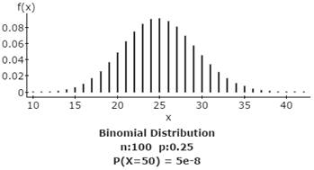
Problem 2. Multiple-choice test
Compute the following binomial probabilities, with n = 100 and p = 0.25.
2a. Find the probability of getting exactly 50 correct answers.
The probability of getting exactly 50 correct answers = 0.00000005
2b. Find the probability of getting at most 40 correct answers.
The probability of getting at most 40 correct answers = 0.99967603

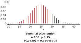
2c. Find the probability of getting less than 30 correct answers.
The probability of getting less than 30 correct answers = 0.85045895
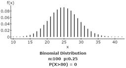
2d. Find the probability of getting more than 80 correct answers.
The probability of getting more than 80 correct answers = 0.0
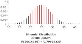
2e. Find the probability of getting between 20 and 30 correct answers.
The probability of getting between 20 and 30 correct answers.
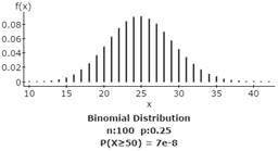
2f. Find the probability of passing the exam (50 or more correct answers).
The probability of passing = 0.0000007
Guided Solution 2
Computer Lab 3A. Activity 2.Find binomial probabilities.
Stat → Calculators → Binomial → Click Standard or Between → Type N in the N box → Type P in the P box → Type X values in the P(X) box → Compute
To copy and paste the binomial probability distribution graph to a Word file:
Options → Copy → Click right mouse button → Copy Image → Paste Special → Device Independent Bitmap
Problem 3. Knee transplant
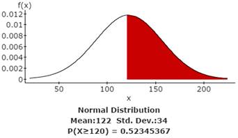
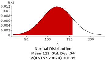
Given that the waiting times for a knee transplant are normally distributed with a mean of 122 days and a standard deviation of 34 days, use StatCrunch to find the following
3a. Find the probability that the waiting time will be at least 120 days.
The probability of waiting at least 120 days = 0.52345367
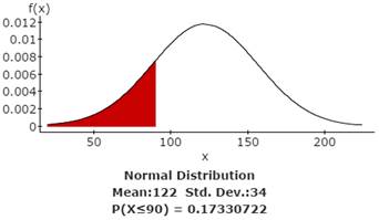
3b. Find the probability that the waiting time will be at most 90 days.
The probability of waiting at most 90 days = 0.17330722
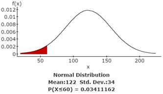
3c. Find the probability that the waiting time will be less than 60 days.
The probability of waiting less than 60 days = 0.03411162
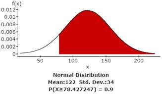
3d. There is a 90% probability that the waiting time will be at least how many days?
There is a 90% probability that the waiting time will be at least 78.427247 days.
3e. There is an 85% probability that the waiting time will be at most how many days?
There is an 85% probability that the waiting time will be at most 157.23874 days.
Guided Solution 3a, b, c
Computer Lab 3B, Activity 1.Find normal probabilities.
Stat → Calculators → Normal → Click Standard or Between → Type the mean → Type the standard deviation → Type the appropriate X values in the P(X) box → Compute
To copy and paste the binomial probability distribution graph to a Word file:
Options → Copy → Click right mouse button → Copy Image → Paste Special → Device Independent Bitmap
Guided Solution 3d, e
Computer Lab 3B, Activity 2.Normal distributions: Find X values.
Stat → Calculators → Normal → Click Standard or Between → Type the mean → Type the standard deviation → Type the given probability in the box after the P(X) box → Compute
Self-Test 4B Solutions
Each Guided Solution below summarizes key Quick Reviews (QR) steps—but not all steps—needed to complete the problem. These QRs will be useful when you are preparing for the computer components of the assignments, midterm exam, and final exam. For more detailed steps, see the relevant Computer Lab and Activity.
QRs are in italics; steps are separated by arrows →.
Problem 1. Population experiment
1a. Create the StatCrunch data file U4_ST_Q1_PopnDist.
Create a StatCrunch data file called U4_ST_Q1_PopnDist, which contains the population probability distribution for the numbers 1, 3, 5, 7, and 9. Copy and paste the probability distribution to the Word file SelfTest4B.
The pasted table is displayed below.
| X | P(X) |
| 1 | 0.2 |
| 3 | 0.2 |
| 5 | 0.2 |
| 7 | 0.2 |
| 9 | 0.2 |
Guided Solution 1a
Computer Lab 1, Activity 2: Open StatCrunch.
Create the variables and enter the values that describe the population distribution:
Type X as the first column variable → Enter the five values of X → Type P(X) as the second column variable → Enter the five values of P(X) → Copy and paste the probability distribution table to the Word file under the Subheading Problem 1a → Select the probability distribution table → Ctrl C → Ctrl V to paste to the Word file.
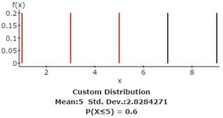
1b. Compute the mean and standard deviation.
Use StatCrunch to display the graph and compute the mean and standard deviation for the population distribution in problem 1a above. Copy and paste the graph and mean and standard deviation from StatCrunch to the Word file SelfTest4B under the subheading Problem 1b. Your results should look the figure below.
Guided Solution 1b
Computer Lab 4A, Activity 1.Find the graph, mean and standard deviation of a population distribution:
With the X and P(X) column variables displayed in the data file:
Stat → Calculators → Custom → In the Values box, select Column variable X → In the Weights box, select the column variable P(X) → Compute
Copy and paste the probability distribution graph to a Word file:
Click right mouse button In StatCrunch Graph window → Copy Image → Paste Special → Device Independent Bitmap
1c. Use StatCrunch to generate 10,000 repetitions.
With the StatCrunch file U4_ST_Q1 data file displayed for the PopnDist, use StatCrunch to generate 10,000 repetitions of the following sampling experiment:
Drawing on the population values 1, 3, 5, 7, and 9, randomly select a sample of 3 values, with replacement, and observe the sample mean. StatCrunch will simulate this experiment 10,000 times, so that 10,000 sample means will be created in one column of the data file. Copy and paste the first five sample means (along with the variable name) from StatCrunch to the Word file SelfTest4B under the subheading Problem 1c.
Your results should look like this:
| mean(Sample(X)) |
| 5.666666666666667 |
| 4.333333333333333 |
| 5 |
| 6.333333333333333 |
| 3 |
Guided Solution 1c
Computer Lab 4A, Activity 3.Approximate the graph, mean, and standard deviation of a sampling distribution of sample means through simulation.
With the Population Distribution variables X and P(X) displayed in the data file:
Data → Sample → Select X column variable → Type sample size → Type number of samples → /Click Sample with replacement → Click Sample all columns at one time → Compute statistic for each sample → Mean(“Sample (X)”)
Copy and paste the first five sample means to the Word file under the subheading problem 1c:
Select the first five sample means → Ctrl C → Ctrl V to paste to the Word file
1d. Compute the overall mean and standard deviation of the 10,000 sample means.
Use StatCrunch to compute the overall mean and standard deviation of the 10,000 sample means that you just generated in 1b above. Copy and paste the Summary Statistics to the Word file SelfTest4B under the subheading Problem 1d.
Your results should look similar to (but not identical to) the figure below.
Summary statistics:
| Column | Mean | Std. dev. |
| mean(Sample(X)) | 4.9972667 | 1.6390631 |
Guided Solution 1d
Computer Lab 4A, Activity 3.With the Mean(Sample(X)) column displayed: Compute Overall mean and standard deviation of the Mean(Sample(X)) Column.
Stat → Summary Stats → Columns → Select Column variable: Mean(Sample(X)) → Select Mean and standard deviation as the statistics → Compute
To copy and paste the summary statistics table to a Word file:
With the Summary statistics table displayed:
Options → Copy → Ctrl A → Ctrl C → Ctrl V
1e. Central Limit Theorem.
Based on the Central Limit Theorem, the mean and standard deviation of the sampling distribution in problem 1d should approximate the population mean and the (population standard deviation/square root of sample size). That is, the mean of the sampling distribution should equal 5 and the standard deviation of the sampling distribution should approximate (2.8284/square root(3)) = 1.6329. As you can see, the mean and standard deviation of the 10,000 sample means displayed in Problem 1d are very close to the Central Limit values.
1f. Create a relative frequency histogram for the 10,000 sample means.
Use StatCrunch to create a relative frequency histogram for the 10,000 sample means you generated in Problem 1c above. Copy and paste the relative frequency histogram from StatCrunch to the Word file SelfTest4B under the subheading Problem 1f. Your results should look similar to (but not identical to) the figure below.

Guided Solution 1f
Computer Lab 4A, Activity 3.With the Mean(Sample(X)) column displayed, create a relative frequency histogram of the sampling distribution of the means:
Graph → Histogram → Select Column variable: Mean(Sample(X)) → In the Type box: Relative Frequency → Compute
1g. Note that the shape of the relative frequency of the 10,000 sample means approximates a normal distribution, as suggested by the Central Limit Theorem.
Problem 2. Exercise 45 from Elementary Statistics, 6th edition
2a. Construct a 90% confidence interval.
Open the StatCrunch data file EX6_1-45.txt in StatCrunch. Use StatCrunch to construct a 90% confidence interval for the mean number of minutes that adults spend watching TV using a DVR, each day. Copy and paste the StatCrunch confidence interval table created (as displayed below) to the Word file SelfTest4B under the subheading Problem 2a.
90% confidence interval results:
μ: Mean of variable
Standard deviation = 4.3
| variable | n | Sample Mean | Std. Err. | L. Limit | U. Limit |
| Times (in minutes) | 20 | 24.1 | 0.96150923 | 22.518458 | 25.681542 |
Guided Solution 2a
Computer Lab 4A, Activity 4.Compute confidence intervals for the population mean: population standard deviation known (given original sample data).
With the appropriate column variable (sample data) displayed in the data file:
Stat → Z Stats → One Sample → With Data → Select Column variable → Type standard deviation → Select Confidence interval option → Type Confidence level → Compute
2b. Construct a 99% confidence interval.
With the StatCrunch data file EX6_1-45.txt open, use StatCrunch to construct a 99% confidence interval for the mean number of minutes that adults spend watching TV using a DVR, each day. Copy and paste the StatCrunch Confidence interval table created (as displayed below) to the Word file SelfTest4B under the subheading Problem 2b.
99% confidence interval results:
μ: Mean of variable
Standard deviation = 4.3
| variable | n | Sample Mean | Std. Err. | L. Limit | U. Limit |
| Times (in minutes) | 20 | 24.1 | 0.96150923 | 21.623316 | 26.576684 |
Guided Solution 2b
Computer Lab 4A, Activity 4.Compute confidence intervals for the population mean: population standard deviation known (given original sample data).
With the appropriate column variable (sample data) displayed in the data file:
Stat → Z Stats → One Sample → With Data → Select Column variable → Type standard deviation → Select Confidence interval option → Type confidence level → Compute
2c. What can you conclude regarding the relationship between the confidence level and the width of the confidence interval?
The larger the confidence level, the wider the confidence interval.
Problem 3. Exercise 30 from Elementary Statistics, 6th edition
3a. Construct a 98% confidence interval.
Open the StatCrunch data file EX6_2-30.txt in StatCrunch. Use StatCrunch to construct a 98% confidence interval for the mean annual earnings of registered nurses. Copy and paste the StatCrunch Confidence Interval Table created to the Word file SelfTest4B under the subheading Problem 3a, as displayed below.
98% confidence interval results:
μ: Mean of variable
| variable | Sample Mean | Std. Err. | DF | L. Limit | U. Limit |
| Annual earnings (in dollars) |
65588.725 | 1870.2041 | 39 | 61051.906 | 70125.544 |
Guided Solution 3a
Computer Lab 4A, Activity 5.Compute confidence intervals for the population mean: population standard deviation unknown (given original sample data).
With the appropriate column variable (sample data) displayed in the data file:
Stat → T Stats → One Sample → With Data → Select Column variable → Select Confidence interval option → Type confidence level → Compute
3b. Test the claim.
Suppose the president of the nurses’ union recently complained that the average annual salary for registered nurses is below $60,000. Test this claim with the confidence interval that you just constructed.
According to the confidence interval, we are 98% confident that the average annual earnings for registered nurses is between $61,051.906 and $70,125.544, which is significantly above the average annual income that the union is claiming. There is less than a 2% chance that the union claim is valid.
3c. Should you have tested first?
In constructing the confidence interval based on the sample of earnings for 40 randomly elected registered nurses, should you have first tested to see if the sample of earnings comes from a normally distributed population?
No need to conduct the normality test, as the sample size exceeds 30 nurses.
Problem 4. Exercise 50 from Elementary Statistics, 6th edition
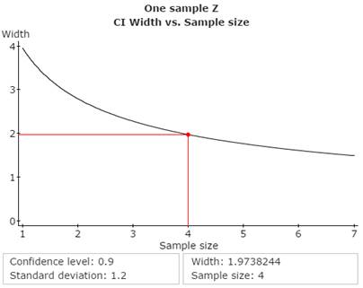
4a. Determine the minimum sample size.
Use StatCrunch to determine the minimum sample size required to construct a 90% confidence interval for mean age with a maximum tolerable error of 1 year (E). Copy and paste the StatCrunch Confidence Interval Width window (as displayed below) to the Word file SelfTest4B under the subheading Problem 4a.
Guided Solution 4a
Computer Lab 4A, Activity 6.Find the minimum sample size to estimate a population mean. With a new StatCrunch data file displayed:
Stat → Z Stats → One Sample → Power → Sample Size → Confidence interval width tab → Type confidence level → Type standard deviation → Type Width (2×Error) → Compute
4b. Determine the minimum sample size.
Use StatCrunch to determine the minimum sample size required to construct a 99% confidence interval with a maximum tolerable error of 1 year (E). See key steps in Problem 4a.
Minimum required sample size is 10 students.
4c. Which level of confidence requires a larger sample size (for the same tolerable error)?
The higher the level of confidence required, the larger the minimum required sample size (for the same tolerable error).
Problem 5. Exercise 16 from Elementary Statistics, 6th edition
According to a survey of 2303 adults, 734 believe in UFOs (unidentified flying objects). Use StatCrunch to construct a 90% confidence interval for the population proportion of adults who believe in UFOs. Copy and paste the StatCrunch Confidence Interval Table (as below) created to the Word file SelfTest4B under the subheading Problem 5.
90% confidence interval results:
p: Proportion of successes
Method: Standard-Wald
| Proportion | Count | Total | Sample Prop. | Std. Err. | L. Limit | U. Limit |
| p | 734 | 2303 | 0.31871472 | 0.0097099858 | 0.30274321 | 0.33468623 |
Guided Solution 5
Computer Lab 4A, Activity 7.Compute a confidence interval for the population proportion.
With a new StatCrunch data file displayed:
Stat → Proportion Stats → One Sample → With Summary → Type number of successes → Type number of observations → Perform: Confidence intervals for P → Type confidence level → Compute
Problem 6. Find the sample size to estimate the population proportion, when no preliminary studies exist.
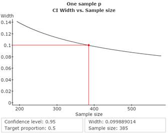
6a. Estimate with 95% confidence when no preliminary studies exist.
You wish to estimate, with 95% confidence, the population proportion of adults who prefer chocolate ice cream over all other flavours. Your estimate must be within 5% of the population proportion. Find the minimum sample size required, when no preliminary studies exist. Copy and paste the StatCrunch Confidence Interval Width window (shown below) to the Word file SelfTest4B, under the subheading Problem 6a.
Guided Solution 6a
Computer Lab 4A, Activity 8.Find the minimum sample size to estimate a population proportion.
With a new StatCrunch data file displayed:
Stat → Proportion Stats → One Sample → Power → Sample Size → Confidence Interval Width → Type confidence level → Type target proportion → Type Width (2×Error) → Compute
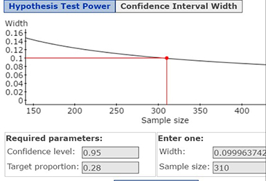
6b. Estimate with 95% confidence when a preliminary study indicates a proportion of 0.28.
You wish to estimate, with 95% confidence, the population proportion of adults who prefer chocolate ice cream over all other flavours. Your estimate must be within 5% of the population proportion. Find the minimum sample size required, when a preliminary study indicates a proportion of 0.28. Copy and paste the StatCrunch Confidence Interval Width window (as displayed below) to the Word file SelfTest4B under the subheading Problem 6b.
Guided Solution 6b
Computer Lab 4A, Activity 8.Find the minimum sample size to estimate a population proportion.
With a new StatCrunch data file displayed:
Stat → Proportion Stats → One Sample → Power → Sample Size → Confidence interval width tab → Type confidence level → Type Target Proportion → Type Width (2×Error) → Compute
Problem 7. Zoeys: Hypothesis Test
7a. Test the hypothesis.
Open the StatCrunch data file Zoeys located in the StatCrunch group folder “AU Math216 2020”. Test the hypothesis that the population mean family income for Zoeys customers exceeds $5000 a month at a 5% level of significance. Use the four-step P‑value approach. Copy and paste the Hypothesis Test Results window from StatCrunch to the Word file SelfTest4B under the subheading Problem 7a under Step 2 of the test.
| Step 1. | Specify the hypotheses: |
||||||||||||
| Step 2. | Use StatCrunch to compute the appropriate Test Statistic and related P‑value
|
||||||||||||
| Step 3. | As the P‑value = 0.0076 is less than alpha = 0.05, reject HO. |
||||||||||||
| Step 4. | The sample does support the claim that the mean family income exceeds $5000 per month for Zoeys customers. |
Guided Solution 7a
Computer Lab 1, Activity 5.Open a data file saved in a StatCrunch group folder at the StatCrunch website
www.StatCrunch.com → Sign in → My StatCrunch → Explore → Groups
Computer Lab 4B, Activity 3.Hypothesis tests for the population mean with population standard deviation unknown—One sample case—Four-step P‑value approach.
Use StatCrunch to compute the appropriate Test Statistic and related P‑value: Given One Sample Data (Step 2):
Stat → T-Stats → One Sample → With Data → Select Column variable → Select Option: Hypothesis Test for Mean → In HO box: Specify null hypothesis → In HA box: Specify alternate hypothesis → Compute
7b. Key assumption.
The key assumption made is that the sample of incomes comes from a normal population, as the sample size is smaller than 30 customers. By making this assumption, you were able to use the t-test statistic.
7c. Hypothesis test.
Conduct the appropriate hypothesis test to determine if the sample of family incomes comes from a normal population. Use the four-step P‑value approach.
| Step 1. | HO: the population mean income is normally distributed. |
||||||||
| Step 2. | Use StatCrunch to compute the Shapiro-Wilks Test Statistic and related P‑value. Shapiro-Wilk goodness-of-fit results:
|
||||||||
| Step 3. | As the P‑value = 0.1047 exceeds alpha, fail to reject HO. |
||||||||
| Step 4. | The population of customer family incomes is normally distributed, so the hypothesis test you conducted in Problem 7a is valid. |
Guided Solution 7c
Computer Lab 4B, Activity 2. Hypothesis test for the assumption of normality: Step 2 in the four-step P‑value approach.
With a column variable (One Sample) displayed in a StatCrunch data file:
Stat → Goodness-of-fit → Normality test → With Data → Select Column variable → Select Shapiro-Wilk
Problem 8. Zoeys: Level of Significance
With the StatCrunch data file Zoeys open, use the four-step P‑value approach to test whether the population proportion of Zoeys customers that frequently use Zoeys coupons is at least 50% with a level of significance of 5%.
| Step 1. | HO: Population proportion is greater than or equal to 0.50. |
||||||||||||||
| Step 2. | Use StatCrunch to compute the appropriate test statistic and related P‑value. Hypothesis test results:
|
||||||||||||||
| Step 3. | As the P‑value = 0.4207 exceeds alpha of 0.05, do not reject HO. |
||||||||||||||
| Step 4. | At least 50% of the population proportion of Zoeys customers frequently use Zoeys coupons. |
Guided Solution 8
Computer Lab 4B, Activity 4. Hypothesis tests involving a single population proportion.
One Sample Case: Four-step P‑value approach, Step 2.
Use StatCrunch to compute the appropriate Test Statistic and related P‑value: Given one sample data
with a column variable (one sample) displayed in a StatCrunch data file:
Stat → Proportion Stats → One Sample → With Data → Select Column → variable → Type Success value → Option: Hypothesis test for P → Specify the null hypothesis → Specify the alternate hypothesis → Compute
Self-Test 5B Solutions
Each Guided Solution below summarizes key Quick Reviews (QR) steps—but not all steps—needed to complete the problem. These QRs will be useful when you are preparing for the computer components of the assignments, midterm exam, and final exam. For more detailed steps, see the relevant Computer Lab and Activity.
QRs are in italics; steps are separated by arrows →.
Problem 1. Exercise 21 from Elementary Statistics, 6th edition
1a. Use the four-step P‑value approach to test whether the mean reading scores under the new curriculum exceeds the mean reading scores under the old curriculum at a 10% level of significance.
Open the StatCrunch file Ex8_2-21.txt in the Math 216 groups folder in StatCrunch. Use the four-step P‑value approach to test whether the mean reading scores under the new curriculum exceed the mean reading scores under the old curriculum at a 10% level of significance. Assume equal population variances when conducting the test (i.e., select the pooled variance option). Copy and paste the Hypothesis Test Results window from StatCrunch to the Word file SelfTest5B under the subheading Problem 1a under Step 2 of the test as shown below.
| Step 1. | Let μ1 be the mean reading scores under the old curriculum. HO: μ1 greater than or equal to μ2 |
||||||||||||
| Step 2. | Use StatCrunch to compute the appropriate Test Statistic and related P‑value. Hypothesis test results:
|
||||||||||||
| Step 3. | As the P‑value = 0.0001 is less than = 0.10, reject HO. |
||||||||||||
| Step 4. | The sample does support the claim that the mean reading scores under the new curriculum exceed the mean reading scores under the old curriculum for third grade students. |
Guided Solution 1a
Computer Lab 1, Activity 5.Open a data file saved in a StatCrunch Group Folder at the StatCrunch website.
www.StatCrunch.com → Sign in → My StatCrunch → Explore → Groups
Computer Lab 5, Activity 2.Test hypotheses involving two population means—wo independent samples—population standard deviations unknown:
Stat → T-Stats → Two Sample → With Data → Select Sample 1 → Select Sample 2 → If variances equal: Select Pooled Variance box → Select Hypothesis Test option → Specify Hypothesis → Compute
1b. What assumption did you make in conducting the hypothesis test in 1a above?
Two assumptions were made: that each of the two sample reading times comes from a normal population; that the two sample reading times come from populations with equal variances.
1c. Conduct the appropriate hypothesis test.
Conduct the appropriate hypothesis test to determine if the each of the two samples of reading scores comes from a normal population. Use the four-step P‑value approach. Copy and paste the Hypothesis Test Results window from StatCrunch to the Word file SelfTest5B under the subheading Problem 1c under Step 2 of the test, as follows. Apply the Shapiro-Wilk test to each of the two samples of reading scores.
| Step 1. | For each sample of scores: |
||||||||||||
| Step 2. | Use StatCrunch to compute the Shapiro-Wilk test statistic and related P‑value for both the old and new curriculum sample reading scores. The Hypothesis Test Results window should display as follows. Shapiro-Wilk goodness-of-fit results:
As described in the above figure: |
||||||||||||
| Step 3. | Make a decision based on comparing the P‑value with the level of significance, alpha, as follows: |
||||||||||||
| Step 4. | It is reasonable to assume that both samples come from normal populations. |
Guided Solution 1c
Computer Lab 4B, Activity 4.Hypothesis test for the assumption of normality: Step 2 in the four-step P‑value approach
Stat → Goodness-of-fit → Normality Test → With Data → Select Column variables → Select Shapiro-Wilk → Compute
1d. Conduct the appropriate hypothesis test, at alpha = 0.05.
Conduct the appropriate hypothesis test, at alpha = 0.05, to determine if the two samples of reading scores come from populations with equal variances. Use the four-step P‑value approach. Copy and paste the Hypothesis Test Results window from StatCrunch to the Word file SelfTest5B under the subheading Problem 1d under Step 2 of the test.
| Step 1. | HO: Variance of Population 1 Equals Variance of Population 2 |
||||||||||||
| Step 2. | Use StatCrunch to compute the F-statistic and related P‑value as follows: Hypothesis test results:
|
||||||||||||
| Step 3. | Make a decision based on comparing the P‑value with the level of significance, alpha. As the P‑value = 0.2638 exceeds alpha, fail to reject HO. |
||||||||||||
| Step 4. | Both samples of reading scores come from populations with equal variances. |
Guided Solution 1d
Computer Lab 4B, Activity 1.Equal Variances Test: Test the hypothesis that two samples come from populations that have equal variances: Four-step P‑value approach, Step 2.
Stat → Variance Stats → Two Sample → With Data → Select Sample 1 → Select Sample 2 → Select Hypothesis Test Option → Select Two Tailed Variance Test → Compute
1e. Construct two separate 90% confidence intervals.
Use StatCrunch to construct two separate 90% confidence intervals: one interval based on the sample of reading scores from the old curriculum, and the second interval based on the sample of reading scores from the new curriculum. Copy and paste both confidence intervals from StatCrunch to the Word file SelfTest5B under the subheading Problem 1e as shown below.
90% confidence interval results:
μ: Mean of variable
| Variable | Sample Mean | Std. Err. | DF | L. Limit | U. Limit |
| Old curriculum | 56.684211 | 1.5968768 | 18 | 53.915125 | 59.453296 |
| New curriculum | 67.4 | 1.8027756 | 24 | 64.315663 | 70.484337 |
Guided Solution 1e
Computer Lab 4A, Activity 5.Compute confidence intervals for the population mean— Population Standard deviation unknown (given sample data):
Stat → T Stats → One Sample → With Data → Select Column variables → Select Confidence interval option → Type confidence level → Compute
1f. Do the two confidence intervals created support your hypothesis test conclusion in Problem 1a?
Yes, as the entire confidence interval estimate for the mean reading scores for the new curriculum is entirely above the entire confidence interval estimate for the mean reading scores for the old curriculum (with no overlap between the two intervals). This supports the conclusion in Problem 1a, that the mean reading scores under the new curriculum exceed the mean reading scores under the old curriculum for third grade students.
Problem 2. Exercise 19 from Elementary Statistics, 6th edition
2a. Test whether eating the new cereal daily lowers mean blood cholesterol levels at a 5% level of significance.
Use the four-step P‑value approach to test whether eating the new cereal daily lowers the mean blood cholesterol levels at a 5% level of significance. Copy and paste the Hypothesis Test Results window from StatCrunch to the Word file SelfTest5B under the subheading Problem 2a under Step 2 of the test.
| Step 1. | Specify the hypotheses: |
||||||||||||
| Step 2. | Use StatCrunch to compute the appropriate Test Statistic and related P‑value. Hypothesis test results:
Differences stored in column, Differences. |
||||||||||||
| Step 3. | Make a decision based on comparing the P‑value with the level of significance, alpha, as follows: |
||||||||||||
| Step 4. | The sample data does not support the manufacturer’s claim that the new cereal lowers blood cholesterol levels. |
2b. What key assumption was made when you tested the manufacturer’s claim in Problem 2a?
In conducting the pairs test in Problem 2a, you assumed that the sample of differences (the d’s) come from a population of differences that is normally distributed.
2c. At the 5% level of significance, test the hypothesis that the sample of differences comes from a population of differences that is normally distributed.
| Step 1. | HO: the population of differences is normally distributed. |
||||||||
| Step 2. | Use StatCrunch to compute the Shapiro-Wilk Test Statistic and related P‑value for the sample of differences, displayed in the data file column Differences. Shapiro-Wilk goodness-of-fit results:
|
||||||||
| Step 3. | Make a decision based on comparing the P‑value with the level of significance, alpha, as follows: |
||||||||
| Step 4. | The sample of differences used in testing the manufacturer’s claim does come from a normal population. As a result, you can use the T-Stat in testing the effectiveness of the new cereal in reducing cholesterol levels as you did in Problem 1a (where you found that the evidence did not support the manufacturer’s claim). |
Guided Solution 2c
Computer Lab 4B, Activity 4.Hypothesis test for the assumption of normality: Step 2 in the four-step P‑value approach.
Stat → Goodness-of-fit → Normality Test → With Data → Select Column variables → Select Shapiro-Wilk → Compute
Problem 3. Exercise 7 from Elementary Statistics, 6th edition
At the 1% level of significance, can you support the claim that there is a difference in the proportion of subjects who feel mostly better between the groups who used the magnetic insoles versus non-magnetic insoles? Use the four-step P‑value approach. Copy and paste the Hypothesis Test Results window from StatCrunch to the Word file SelfTest5B under the subheading Problem 3 under Step 2 of the test, as displayed below.
| Step 1. | Let p1 = population proportion of subjects with magnetic insoles feeling mostly better. HO: p1 − p2 = 0 |
||||||||||||||||||
| Step 2. | Use StatCrunch to compute the appropriate Test Statistic and related P‑value Hypothesis test results: |
||||||||||||||||||
|
|||||||||||||||||||
| Step 3. | Make a decision based on comparing the P‑value with the level of significance, alpha, as follows: |
||||||||||||||||||
| Step 4. | The sample data does not support the claim that there is a difference between the subjects’ response to wearing the magnetic insoles versus the non-magnetic insoles. |
||||||||||||||||||
Guided Solution 3
Computer Lab 5, Activity 4.Test hypotheses involving two population proportions with summary data:
Stat → Proportion Stats → Two Sample → With Summary → In Sample 1 section: Type # successes and type # observations → In Sample 2 section: Type # successes and type # observations → Select Hypothesis Test option → Specify Hypothesis → Compute
Problem 4. Zoeys: Another Hypothesis Test
4a. Test the hypothesis.
Open the StatCrunch data file Zoeys. At a 5% level of significance, that the population mean amount spent per month by the female customers at Zoeys exceeds that the population mean amount spent per month by the male customers at Zoeys. Use the four-step P‑value approach. Copy and paste the Hypothesis Test Results window from StatCrunch to the Word file SelfTest5B under the subheading Problem 4a under Step 2 of the test. Use the pooled variance option when conducting this test.
| Step 1. | Specify the hypotheses: HO: μ1 less than or equal to μ2 |
||||||||||||
| Step 2. | Use StatCrunch to compute the appropriate Test Statistic and related P‑value Hypothesis test results:
|
||||||||||||
| Step 3. | As the P‑value = 0.0001 is less than alpha = 0.05, reject HO |
||||||||||||
| Step 4. | The sample supports the claim that the population mean amount spent per month by the female customers at Zoeys exceeds the population mean amount spent per month by the male customers at Zoeys. |
Guided Solution 4a
Computer Lab 1, Activity 5.Open a data file Saved in a StatCrunch Group Folder at the StatCrunch Website
www.StatCrunch.com → Sign in → My StatCrunch → Explore → Groups
Computer Lab 5, Activity 2.Test hypotheses involving two population means-two independent samples-population standard deviations unknown:
Stat → T-Stats → Two Sample → With Data → Select Sample 1: Values In box: Spend: Where box: "Recode(Gender)" = Female → Select Sample 2: Values In box: Spend: Where box: "Recode(Gender)" = Male → If Variances Equal: Click on Pooled Variance box → Select Hypothesis Test Option → Specify Hypothesis → Compute
4b. What assumptions did you make in conducting the hypothesis test in 4a above? You assumed that the two spending subset samples (amounts spent by females and males) come from populations with equal variances. You also assumed that each of the two spending subset samples (amounts spent by females and males) come from normal populations.
4c. Conduct the appropriate hypothesis test, at alpha = 0.05, to determine if the each of the two subset samples - amounts spent by the female customers and amounts spent by the male customers - comes from populations with equal variances.
| Step 1. | Specify the hypotheses |
||||||||||||
| Step 2. | Use StatCrunch to compute the F-statistic and related P‑value as follows: Hypothesis test results:
|
||||||||||||
| Step 3. | Make a decision based on comparing the P‑value with the level of significance, |
||||||||||||
| Step 4. | State your conclusion: Both subset spending amounts samples come from populations with equal variances. |
Guided Solution 4c
Computer Lab 4B, Activity 1.Equal Variances Test: Test the hypothesis that two samples come from populations that have equal variances: Four-step P‑value approach, Step 2.
Stat → Variance Stats → Two Sample → With Data → Select Sample 1: Values In box: Spend: Where box: "Recode(Gender)" = Female → Select Sample 2: Values In box: Spend: Where box: "Recode(Gender)" = Male → Select Hypothesis Test Option → Select Two Tailed Variance Test → Compute
4d. Conduct the appropriate hypothesis test to determine if each of the two subset samples - amounts spent by the female customers and amounts spent by the male customers - comes from normal populations.
| Step 1. | Specify the hypotheses for each of the two subset samples of spending amounts: |
||||||||||||
| Step 2. | Use StatCrunch to compute the Shapiro-Wilk Test Statistic and related P‑value for both of the spending subsets. The Hypothesis Test Results window should display as follows. Shapiro-Wilk goodness-of-fit results:
|
||||||||||||
| Step 3. | Make a decision based on comparing the P‑value with the level of significance, alpha, as follows: |
||||||||||||
| Step 4. | State your conclusion. Since it appears that the sample of spending amounts made by the male customers does not come from a normal population, we cannot use the T-Stat in conducting the hypothesis test in Problem 1a. with the current data collected. One option is to sample additional Zoeys customers to the point of having each subset sample size exceed 30 customers |
Guided Solution 4d
Computer Lab 4B, Activity 4.Hypothesis test for the assumption of normality: step two in the four-step P‑value approach:
Stat → Goodness-of-fit → Normality Test → With Data → Select Column variable: Spend → In the Group By box: Select Recode(Gender) → Select Shapiro-Wilk → Compute
Problem 5. Zoeys: Population Proportion
With the StatCrunch data file Zoeys open, use the four-step P‑value approach to test whether the population proportion of Zoeys female customers that frequently use Zoeys coupons exceeds the population proportion of Zoeys male customers that frequently use Zoeys coupons, with a level of significance of 5%.
| Step 1. | Specify the hypotheses: |
||||||||||||||||||
| Step 2. | Use StatCrunch to compute the appropriate Test Statistic and related P‑value. Hypothesis test results: |
||||||||||||||||||
|
|||||||||||||||||||
| Step 3. | Make a decision based on comparing the P‑value with the level of significance, alpha, as follows: |
||||||||||||||||||
| Step 4. | The sample data does support the claim that the population proportion of Zoeys female customers who frequently use Zoeys coupons exceeds the population proportion of Zoeys male customers who frequently use Zoeys coupons. |
||||||||||||||||||
Guided Solution 5
Computer Lab 5, Activity 4.Test hypotheses involving two population proportions with the appropriate column variable—summary data:
Stat → Proportion Stats → Two Sample → With Summary →
Sample 1 Values box: Recode(Coupon) → Success: Freq → Where: "Recode(Gender)" = Female →
Sample 1 Values box: Recode(Coupon) → Success: Freq → Where: "Recode(Gender)" = Male →
Select Hypothesis Test Option → Specify One Tailed Test → Compute
Self-Test 6B Solutions
Each Guided Solution below summarizes key Quick Reviews (QR) steps—but not all steps—needed to complete the problem. These QRs will be useful when you are preparing for the computer components of the assignments, midterm exam, and final exam. For more detailed steps, see the relevant Computer Lab and Activity.
QRs are in italics; steps are separated by arrows →.
Problem 1. Exercise 23 from Elementary Statistics, 6th edition
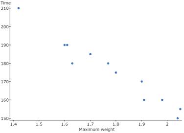
1a. Use StatCrunch to create a Scatterplot with Weight on the X-axis and Time on the Y-axis.
Open the eText data file Ex9_1-23.txt in StatCrunch.
Guided Solution 1a
Computer Lab 6A, Activity 1.Conduct correlation analysis.
Create a Scatterplot based on two variables:
Graph → Scatterplot → Select the X Column variable → Select the Y Column variable → Compute
1b. Does the plot suggest a positive or negative correlation between Weight and Time?
According to the Scatterplot in 1a above, there appears to be quite a strong negative linear correlation between weight and time. As the weight increases, the sprint time decreases.
1c. Correlation Coefficient, r, between Time and Maximum weight
r = −0.9745954
Guided Solution 1c
Computer Lab 6A, Activity 1.Conduct correlation analysis.
Compute the correlation coefficient between two variables:
Stat → Summary Stats → Correlation → Select the two Column variables → Compute
1d. Interpret the correlation coefficient.
A correlation coefficient equal to −0.9745954 means that there is a strong negative linear relationship between Weight and Time.
1e. Conduct the t-test.
At a 5% level of significance use StatCrunch to conduct the t-test to see if the population correlation coefficient, ρ, between Weight and Time, is significantly different from zero. Use the four-step P‑value approach.
| Step 1. | HO: the population correlation coefficient ρ = 0 |
| Step 2. | Correlation between Time and Maximum weight is: −0.9745954(< 0.0001); |
| Step 3. | As the P‑value = 0.0001 is less than alpha = 0.05, reject HO. |
| Step 4. | Weight is significantly correlated with Time (sprint performance). |
Guided Solution 1e
Computer Lab 6A, Activity 1.Conduct correlation analysis.
Compute the P‑value for two tailed hypothesis test regarding correlation:
Stat → Summary Stats → Correlation → Select the two Column variables → Select Option: Two Sided P‑value → Compute
Problem 2. Nurses’ Salaries
The experience (in years) of 14 registered nurses and their annual salaries (in thousands of dollars) is displayed in the data file RNurse_Salaries.txt, available in the StatCrunch Group AU Math216 2020.
2a. Find the equation of the linear regression line.
Find the equation of the linear regression line with Years of experience being the independent variable and Annual salary being the dependent variable. Copy and paste the first screen of the Simple Linear Regression Results window from StatCrunch as shown in Figure 1 below. Note that the output in Figure 1 will be used to answer Problems 2a, 2b, 2c, 2d, 2e, 2f, and 2g.
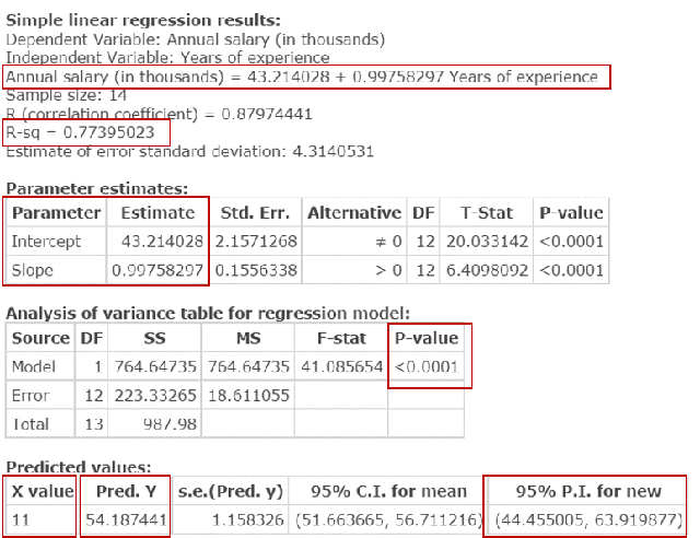
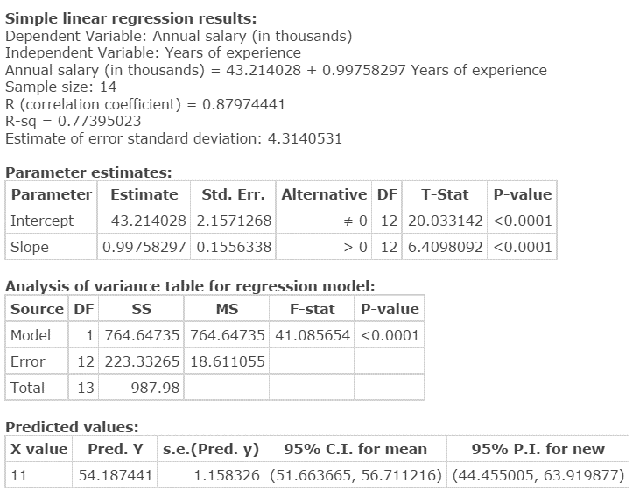
Figure 1. Screen 1 of the Regression Results window. Equation of the linear regression line is: Annual Salary = 43.214028 + 0.99758297 Years Experience
Guided Solution 2a
Computer Lab 6A, Activity 2.Conduct linear regression analysis:
Regression Equation, Fitted Plot, Coefficient of Determination, Significance Test, Prediction Intervals
Stat → Regression → Simple Linear → Select X column variable → Select Y column variable → Perform Hypothesis Test → Specify HA: Slope greater than zero → Type X and Level for Prediction of Y → Select Fitted Line Plot option for graphs → Compute
2b. Plot the regression line along with the Scatterplot.
Copy and paste the graph created from StatCrunch in the second screen of the Simple Linear Regression Results window as shown in Figure 2 below.
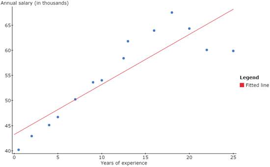
Figure 2. Fitted regression plot.
2c. What does the slope of the regression line suggest about the relationship between the two variables?
The slope from the solution to 2a is 0.99758297. As the slope is positive, this implies that the regression line is upward sloping so that, as Years of Experience increases, Annual Salary increases.
2d. Compute the Coefficient of Determination, r-squared.
Based on the Simple Linear Regression Results window pasted from 2a above, the Coefficient of Determination, r-squared = 0.77395.
2e. Interpretation of Coefficient of Determination = 0.77395.
77% of the variation in annual salary of registered nurses can be explained by the variation in years of experience.
2f. At the 5% level of significance, test to see if the slope of the regression line significantly exceeds zero. Use the four-step P‑value approach.
Hypothesis Test re Slope of Regression Line: Four-step P‑value approach:
| Step 1. | HO: M = 0 (Slope = 0) |
| Step 2. | Use StatCrunch to compute the Test Statistic and related P‑value. Note that the P‑value = 0.0001 from Problem 2a above. |
| Step 3. | Make a decision based on comparing the P‑value with the level of significance, alpha: |
| Step 4. | The slope of the Regression Line significantly exceeds 0. There is a significant positive linear relationship between Years of experience and Annual salary. You can use the Simple Linear Regression Equation to predict Annual salary based on given Years of experience. |
2g. Construct a 95% prediction interval for the annual salary for a registered nurse with 11 years of experience.
Based on the Simple Linear Regression Results window pasted from 2a above, the 95% prediction interval is: 44.45500 to 63.9198 in thousands.
2h. Single prediction estimate for the annual salary for a registered nurse with 11 years of work experience.
Based on the Simple Linear Regression Results window from 2a above, the single estimate for the annual salary for a registered nurse with 11 years of experience is 54.187441 thousands or $54,1874.41.
Problem 3. Funland
3a. Create a contingency table.
Use StatCrunch to create a contingency table for the Survey Responses in the Funland data file, with Marital displayed as the row variable, and Pass displayed as the column variable. Copy and paste the contingency table as displayed below. Note that the output in in the tables below will be used to answer Problems 3a, 3b, 3c, and 3d.
Contingency table results:
Rows: Recode(Marital)
Columns: Recode(Pass)
| Cell format |
| Count (Row percent) |
| No | Yes | Total | |
| Married | 1 (5.56%) |
17 (94.44%) |
18 (100%) |
| Single | 7 (100%) |
0 (0%) |
7 (100%) |
| Total | 8 (32%) |
17 (68%) |
25 (100%) |
Chi-Square test:
| Statistic | DF | Value | P‑value |
| Chi-square | 1 | 20.659722 | < 0.0001 |
Warning: Over 20% of cells have an expected count less than 5. Chi-Square suspect.
Guided Solution 3a
Computer Lab 6B, Activity 1.Conduct chi-square independence test.
Stat → Tables → Contingency → With Data → Select the row variable → Select the column variable → Display Row Percent → Click Chi-Square Test of Independence → Compute
3b. Determine whether the variables Marital and Pass are independent or related.
Use the contents of the Chi-Square Test Table to conduct a test of hypothesis, at a 5% level of significance to determine whether the variables Marital and Pass are independent or related. Use the four-step P‑value approach as follows, with the Chi Square Test statistic and P‑value shown in Step 2.
| Step 1. | HO: Marital and Pass are independent. |
| Step 2. | Test Statistic = Chi-Square = 20.659722 and related P‑value is less than 0.0001. |
| Step 3. | As the P‑value is less than the level of significance of 0.05, reject HO. |
| Step 4. | In the Funland survey, there is a significant relationship between marital status and the tendency to purchase a monthly pass. |
3c. Describe the relationship between the variables Recode(Marital) and Recode(Pass).
Based on the row percentages displayed in the second column of the contingency table, while 94.44% of the married customers surveyed said Yes to purchasing the monthly pass, only 0% of the single customers surveyed said Yes to purchasing the monthly pass. In general, married customers tend to be significantly more inclined to purchase the monthly pass than single customers.
3d. Comment on the expected frequency assumption underlying the Chi-square test used in independence test used in Problem 1b.
As displayed in the bottom of the chi-square table warning: “Over 20% of cells have an expected count less than 5”. This warning indicates that we cannot rely on the results of the Chi-Square test of independence conducted in Problem 3c.
Problem 4. Exercise 14 from Elementary Statistics, 6th edition
4a. Conduct an ANOVA test.
Open the eText data file Ex10_4-14.txt in StatCrunch. Conduct an ANOVA test of hypothesis to see if at least one city’s mean sale price is different from the mean sales prices in the other two cities surveyed, at a 10% level of significance.
| Step 1. | Specify the hypotheses: HO: u1 = u2 = u3 |
||||||||||||||||||||||||||||||||||||||||||||
| Step 2. | Use StatCrunch to compute the appropriate Test Statistic and related P‑value Analysis of Variance results: Column statistics
ANOVA table
Note: Test Statistic = F = 0.96607611 and P‑value = 0.3929 |
||||||||||||||||||||||||||||||||||||||||||||
| Step 3. | Make a decision based on comparing the P‑value with the level of significance, alpha, as follows: |
||||||||||||||||||||||||||||||||||||||||||||
| Step 4. | You cannot conclude that the mean house sale prices between the three cities surveyed. |
Guided Solution 4a
Computer Lab 6B, Activity 2.One way analysis of variance (ANOVA).
Stat → ANOVA → One Way → Select all variables → Compute
4b. Test the assumption of equal variances at a 5% level of significance.
Test the assumption of equal variances at a 5% level of significance. Use the four‑step P‑value approach. Copy and paste the table displaying the Levene’s Test For Homogeneity of Variance under Step 2 of the test.
| Step 1. | HO: σ12 = σ22 = σ32 |
||||||||
| Step 2. | The Test Statistic and related P‑value Levene's Test for Homogeneity of Variance
Note the P‑value = 0.4346 |
||||||||
| Step 3. | As the P‑value exceeds the level of significance of 0.05, do not reject HO. |
||||||||
| Step 4. | You can conclude that the assumption of equal variances is reasonable. |
Guided Solution 4b
Computer Lab 6B, Activity 2.One way analysis of variance (ANOVA).
Stat → ANOVA → One Way → Select all variables → Select Option: Homogeneity of variance → Levene’s Test → Compute
4c. Determine if the samples come from normal populations.
Use the Shapiro-Wilk Test for Normality to determine if each of the three samples in the data file Ex10_4-14.txt appears to come from a normal population. Assume a 5% level of significance for this test. Use the four-step P‑value approach.
| Step 1. | HO: Each population is normally distributed. |
||||||||||||||||
| Step 2. | Use StatCrunch to compute the Shapiro-Wilks Test Statistic and related P‑value. Shapiro-Wilk goodness-of-fit results:
Note: the P‑values for the three samples are: 0.4509, 0.8072, 0.1983 |
||||||||||||||||
| Step 3. | Make a decision based on comparing the P‑value with the level of significance, alpha, as follows: |
||||||||||||||||
| Step 4. | You cannot conclude that the population is not normally distributed (therefore, the assumption of normal population is reasonable) for each of the three samples. |
Guided Solution 4c
Stat → Goodness-of-fit → Normality Test → With Data → Select all variables → In the Test box, select Shapiro-Wilk → Compute