Mathematics 216 Computer-oriented Approach to Statistics
Computer Lab 3A
with Guided Solutions (Technology Manual)
Activity 1. Find the mean and standard deviation of a discrete random variable.
The first section of Chapter 4 of your text focuses on the features of a discrete probability distribution, along with its mean and standard deviation. The next activity uses StatCrunch to compute the mean and standard deviation of a discrete probability distribution.
Task 1. Example 7 from Elementary Statistics, 6th edition
Example 7 Finding an Expected Value

If you buy one of the 1500 available tickets, what is the expected value and standard deviation of the random variable X where X is your dollar gain (after deducting the $2 ticket cost)?
The discrete probability distribution of X, where X is your dollar gain, is shown in Figure 1. Note that (1/1500) = 0.00067 and (1496/1500) = 0.9973.
| Gain, X | $498 | $248 | $148 | $73 | $−2 |
| P(X) | 0.000667 | 0.000667 | 0.000667 | 0.000667 | 0.9973 |
Figure 1. Probability distribution of X, where X is dollar gain from buying a winning raffle ticket
Guided Solution 1a
Create the data file: Example 7: Probability Distribution of X
- Sign in to statcrunch.com.
- Click the menu option Open StatCrunch.
- In the blank data table, replace the variable names Var1 and Var2 with X and P(X).
- Under X, enter the five possible values of X.
Under P(X), enter the five values as in Figure 1. Figure 2 describes the probability distribution in StatCrunch.

Figure 2. Probability distribution in StatCrunch data table
- Click the menu sequence: Data → Save.
- In the Filename box, type Example 7.
- Click Save to save to your My Data folder.
- Keep this data file open for Guided Solution 1b.
Guided Solution 1b
Use StatCrunch to compute the mean and standard deviation for the discrete probability distribution in File Example7_P196.
Here, you will use StatCrunch to compute the Expected Value (Mean) and Standard Deviation for the Probability Distribution displayed in your data table as shown in Figure 3. Note that there are no visible points on the graph for values of X, other than X = −2, because of the very small probabilities related to the other values of X.
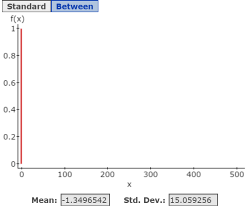
Figure 3. Graph, Mean and Standard Deviation of Probability Distribution for Example 7 P196
- With the data file Example7_P196 open, click the menu sequence Stat → Calculators → Custom.
- In the Values box, select the variable X.
- In the Weights box, select the variable P(X).
- Click Compute to display the graph showing Mean = −1.3496542 and Std. Dev. = 15.059256
Guided Solution 1c
Copy the probability distribution graph into a new Word file called ComputerLab3A.
- Create a new Word file entitled Computer Lab 3A.
- Type its title, ComputerLab3A.
- Below the title, type: Example 7 page 196.
- Below that, copy and paste the Graph, Mean and Standard Deviation of Probability Distribution for Example 7 P196 that you just created in StatCrunch. (For help with copying StatCrunch data, see Copying Materials from StatCrunch.)
- Save the Word file, ComputerLab3A.
Task 2. Interpretation Question: Find the “long run average” gain for the raffle example.
Copy the question below into your ComputerLab3A Word file, below the bottom item:
Consider the weekly raffle, in which 1500 tickets are sold at $2 each for the opportunity to win one of four prizes of $500, $250, $150, and $75. Suppose you bought one raffle ticket every week for a long period of time. What would your average weekly gain be from playing this raffle?
Solution:
Based on your review of the pasted frequency table, type your answers to this question in the solution space provided. (If you need help answering the question, see the Solution that follows.)
Remember to save your Word file, ComputerLab3A.
Solution 2
- Solution: Mean = −1.3496542, which means that over a long period of time you can expect to gain $−1.35 per week (lose $1.350 per week)
Task 3. Find the mean and standard deviation for a game of roulette.
Roulette is a popular game in casinos, exhibitions, and fairs. A roulette wheel contains 38 spaces of equal size. The wheel is spun and a ball randomly lands in one of these spaces. Two spaces are green and have the numbers 0 and 00 on them. The other spaces are numbered from 1 to 36; 18 of these remaining spaces are red, and 18 are black. Various types of bets are made on where the ball will land. A common game is to choose a colour, such as red, and bet a certain amount that the ball will land on any of the 18 red spaces.
Here, you have bet $1 on a red space coming up each time you play roulette. The random variable X will equal your net winnings on one play of this game. If you bet $1 on red and red occurs, then you will win your dollar (X) back plus another dollar, so that X = 1. The probability that you will win equals (18/38) = 0.47368. If you bet $1 on red but the ball lands on green or black, then you lose the dollar and X = −1. The probability that you will lose equals (20/38) = 0.52632. Figure 4 describes the probability distribution for this game of roulette.
| Gain, X | $1 | $−1 |
| P(X) | 0.47368 | 0.52632 |
Figure 4. Probability distribution of roulette game
Guided Solution 3a
Here, you will use StatCrunch to:
- Create a data file of the probability distribution of the roulette game, as displayed in Figure 4.
- Compute the mean and standard deviation for this distribution.
To create the data file: Exercise: Roulette_Red: Probability Distribution of X:
- Sign in to statcrunch.com.
- Select the menu option Open StatCrunch.
- In the blank data table, replace the variable names Var1 and Var2 with X and P(X).
- Under X, enter the two possible values of X, shown in Figure 4.
- Under P(X), enter the two values of P(X), shown in Figure 4.
- Click the menu sequence Data → Save.
- In the Filename box, type Exercise_Roulette_Red.
- Click Save to save to your My Data folder.
- Keep this data file open.
Guided Solution 3b
Use StatCrunch to compute the mean and standard deviation for the roulette probability distribution in the data file Exercise_Roulette_Red
Here, you will use StatCrunch to create the graph and to compute the expected value (mean) and standard deviation for the roulette probability distribution as displayed in Figure 5.
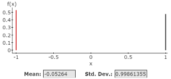
Figure 5. Graph: mean and standard deviation of roulette probability distribution
- With the data file Exercise_Roulette_Red open, click the menu sequence: Stat → Calculators → Custom.
- In the Values box, select the variable X.
- In the Weights box, select the variable P(X).
- Click Compute to display Mean = −0.05264 and Std. Dev. = 0.99861355 as shown in Figure 5.
Guided Solution 3c
Copy the probability distribution into your Word file ComputerLab3A.
- Open the ComputerLab3A Word file.
- Below the bottom item, type the title: Graph, Mean and Standard Deviation of Roulette Probability Distribution.
- Below that, copy and paste the Graph, Mean and Standard Deviation of the Roulette probability distribution created in StatCrunch. (For help with copying StatCrunch data, see Copying Materials from StatCrunch.)
- Save your Word file, ComputerLab3A.
Task 4. Interpretation Question: Find the “long run average” gain for the roulette game.
Copy the question below into your ComputerLab3A Word file, under the bottom item.
You have played the roulette game, betting a dollar on red, a large number of times. Find your expected average dollar gain or loss.
Solution:
Based on your review of the pasted graph, type your answer to this question in the solution space provided. (If you need help answering the question, see the Solution that follows.)
Remember to resave your Word file, ComputerLab3A.
Solution 4
- Solution: Mean = −0.05264, which means that over a long period of time you can expect to lose approximately $−0.05 per game. As with all casino games, the expected gain is negative; this enables the casino company to pay its expenses and make a profit.
Activity 2. Find binomial probabilities.
Here, you will use StatCrunch to compute binomial probabilities.
Task 5. Exercise 21 from Elementary Statistics, 6th edition
Exercise 21. Comfortable Retirement

First, note that this exercise describes a binomial experiment in which:
n = 10
p = 0.51
X = number of workers who are confident of being able to retire comfortably.
Guided Solution 5a
For (a) is exactly two:
P(X is exactly 2) = P(X = 2)
Binomial Probability: P(X = 2)
- Sign in to statcrunch.com.
- Select the menu option Open StatCrunch.
- Click the menu sequence: Stat → Calculators → Binomial. This will display a binomial probabilities window showing the graph of the binomial distribution.
- In the text boxes below the graph:
- in the n box, type 10
- in the p box, type 0.51
in the P(X) box, select = in the first box, and type 2 in the second box. (See Figure 6.)
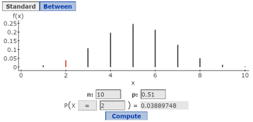
Figure 6. Binomial probabilities window
- Click Compute. This will display the solution P(X = 2) = 0.03889748
Guided Solution 5b
Copy the Binomial Probability Distribution P(X = 2) graph into your Word file, ComputerLab3A.
- Open the ComputerLab3A Word file.
- Below the bottom item, type the title Binomial Probabilities P(X = 2).
- In the next line, copy and paste the binomial probability distribution graph. You will then save this document under the file name ComputerLab3A. (For help with copying StatCrunch data, see Copying Materials from StatCrunch.)
- Save your Word file, ComputerLab3A.
Guided Solution 5c
For (b) more than two:
P(X is more than two) = P(X > 2)
Binomial Probability: P(X > 2)
- With StatCrunch open, click the menu sequence: Stat → Calculators → Binomial.
- In the text boxes below the graph:
- in the n box, type 10.
- in the p box, type 0.51.
- in the P(X) box, select > in the first box, and type in 2 in the second box.
- Click Compute to display the solution P(X > 2) = 0.95199968.
Guided Solution 5d
- Copy the Binomial Probability Distribution P(X > 2) graph into your Word file, ComputerLab3A. Follow the steps in Guided Solution 5b, but type the title Binomial Probabilities P(X > 2).
Guided Solution 5e
For (c) between two and five, inclusive:
P(X is between 2 and 5 inclusive)
Binomial Probability: P(X is between 2 and 5 inclusive)
- With StatCrunch open, click the menu sequence: Stat → Calculators → Binomial.
Near the top of the graph window, click the Between button. (See Figure 7.)
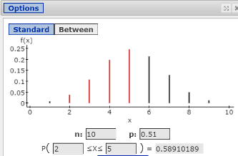
Figure 7. Binomial Probabilities Window: P(X is between 2 and 5 inclusive)
- In the text boxes below the graph:
- in the n box, type 10
- in the p box, type 0.51
- in the P(X) box, select 2 in the first box, and type 5 in the second box. (See Figure 7.)
- Click Compute to display the solution P(X is between 2 and 5 inclusive) = .058910189.
Guided Solution 5f
- Copy the Binomial Probability Distribution P(X is between 2 and 5 inclusive) graph into your Word file, ComputerLab3A. Follow the steps in Guided Solution 5b, but type the title Binomial Probabilities P(X is between 2 and 5 inclusive).
Guided Solution 5g
What if the number of workers confident of a comfortable retirement is at most six? Then:
P(X is at most 6) = P(X ≤ 6)
Binomial Probability: P(X ≤ 6)
- With StatCrunch open, click the menu sequence: Stat → Calculators → Binomial.
- Near the top of the graph window, click the Standard button.
- In the text boxes below the graph:
- in the n box, type 10
- in the p box, type 0.51
- in the P(X) box, select ≤ in the first box, and type in 6 in the second box.
- Click Compute to display the solution P(X ≤ 6) = .81122683.
Guided Solution 5h
- Copy the Binomial Probability Distribution P(X ≤ 6) graph into your Word file, ComputerLab3A. Follow the steps in Guided Solution 5b, but type the title Binomial Probabilities (X ≤ 6).
Guided Solution 5i
What if the number of workers confident of a comfortable retirement is at least four? Then:
P(X is at least 4) = P(X ≥ 4)
Binomial Probability: P(X ≥ 4)
- With StatCrunch open, click the menu sequence: Stat → Calculators → Binomial.
- Near the top of the graph window, click the Standard button.
- In the text boxes below the graph:
- in the n box, type 10
- in the p box, type 0.51
- in the P(X) box, select ≥ in the first box, and type 4 in the second box.
- Click Compute to display the solution P(X ≥ 4) = .84403932.
Guided Solution 5j
- Copy the Binomial Probability Distribution P(X ≥ 4) graph into your Word file, ComputerLab3A. Follow the steps in Guided Solution 5b, but type the title Binomial Probabilities P(X ≥ 4).
Guided Solution 5k
What if the number of workers confident of a comfortable retirement is less than six? Then:
P(X is less than 6) = P(X < 6)
Binomial Probability: P(X < 6)
- With StatCrunch open, click the menu sequence: Stat → Calculators → Binomial.
- Click the Standard button.
- In the text boxes below the graph:
- in the n box, type 10
- in the p box, type 0.51
- in the P(X) box select < in the first box and type in 6 in the second box.
- Click Compute to display the solution P(X < 6) = .59820472.
Guided Solution 5l
- Copy the Binomial Probability Distribution P(X < 6) graph into your Word file, ComputerLab3A. Follow the steps in Guided Solution 5b, but type the title Binomial Probabilities P(X < 6).
Activity 3. Use StatCrunch to simulate the playing of a roulette game. This activity, which includes Task 6 and Task 7 below, is an advanced activity which can be skipped, without affecting student academic performance in this course.
Task 6. Find the long run average of placing a “Street Bet” in a roulette game.
As noted above, a roulette wheel contains 38 equally sized spaces or slots. The wheel is spun and a ball randomly lands in one of these slots. Two slots have numbers 0 and 00 and the other slots are numbered from 1 to 36. Wagers can be made on the slot the ball will land on.
Assume that you have placed a Street Bet. A Street Bet gives you three different numbers for a single wager, with 11 to 1 odds.
For each play of the game, you will bet $5 on the three numbers 11, 12, 13. If the ball lands on one of these numbers, you will receive a net payoff of 11 × 5 = $55, and you will get your $5 back in addition to this net payoff. If the ball does not fall on one of these three numbers, you will lose $5 or receive a net payoff of $−5. If we let the random variable be the net payoff, X, then X will be either $+55 or $−5, for each play of the game.
The StatCrunch data file entitled Street_Roulette has been added to the StatCrunch Group AU Math216 2020. The first variable (column) Slot contains the roulette slot numbers 1 to 36 followed by two zeros. The second variable (column) NetPayoff shows the net payoffs associated with each slot number as described above for the street bet.
Your task is to use StatCrunch to simulate placing the Street Bet 200 times every day for 365 days. StatCrunch will then compute the mean daily net payoff in a new column of the data table. Finally, you will use StatCrunch to compute the mean of these 365 daily mean payoffs, which would be considered a long run average net payoff from placing the Street Bet.
Guided Solution 6a
- Open the StatCrunch File Street_Roulette from the My Groups folder. (For help accessing this resource, see Accessing and Working in StatCrunch on the course home page.)
- You should now see the two variables, Slot and NetPayoff, displayed in the data table, with 38 rows of data.
Guided Solution 6b
Computing the mean daily net payoff from 200 plays per day of the Street Bet for 365 days.
- With the Street_Roulette file open in StatCrunch, click the menu sequence: Data → Sample.
- In the Sample Columns window that displays:
- Using the Ctrl key click select both variables, Slot and NetPayoff.
- In the Sample size box, type 200 (the number of daily plays).
- In the Number of samples box, type 365 (365 days of playing).
- In the Sampling options section, click:
- Sample with replacement
- Sample all columns at one time
- In the Store samples section:
- Compute statistic for each sample.
- In the Build box, type mean(“Sample(NetPayoff)”).
- Under Seeding, select Use fixed seed. See Figure 8.
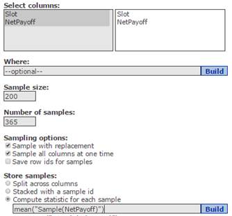
Figure 8. Sample Columns window for 200 roulette plays for 365 days
- Click Compute. This will display a new column/variable, called mean (Sample (NetPayoff)). showing average daily payoffs for 365 days (365 rows). This columns shows the average daily net payoff for each day you played roulette (200 times per day).
Guided Solution 6c
Compute the mean of the daily mean netpayoffs.
- With the new column mean (Sample(NetPayoff)) displayed in StatCrunch, click the menu sequence: Stat → Summary Stats → Columns.
- In the Summary Stats window that displays:
- In the Select Columns box, select the variable mean(Sample(NetPayoff)).
- In the Statistics box, select mean.
- Click Compute to display a mean of −.29287671
Task 7. Interpretation Question: How much was lost or won?
Based on your StatCrunch results, how much, in total, would you have won or lost from playing roulette 200 times per day for 365 days?
Solution:
Solution 7
- Overall, you would have lost $21,379.50 from playing the roulette game a total of 200 × 365 = 73,000 times, that is 73,000 × $−.29287 = $21,379.50.
If you are interested in reading more about roulette and StatCrunch, go to page 6: StatCrunch ACTIVITY: Playing Roulette at https://bgsu.instructure.com/courses/901773/pages/p6-statcrunch-activity-playing-roulette?module_item_id=6369608)
