Mathematics 216 Computer-oriented Approach to Statistics
Computer Lab 6B
with Guided Solutions (Technology Manual)
With the aid of the Guided Solutions, you will use StatCrunch to work through each of the following Activities, which relate to two topics in Chapter 10 of your eText: Chi‑square independence test, and One way analysis of variance.
Activity 1. Chi-Square Independence Test
Figure 1 describes a survey questionnaire that was completed by all 210 staff working at a small college. The survey responses are in the StatCrunch data file College_Giving, in the Math 216 groups folder.
| Please check the survey codes that apply to you below. | Variable | Text Code |
| 1. Please check your gender. | Gender | |
| ☐ male | ______ M | |
| ☐ female | ______ F | |
| 2. Have you have engaged in volunteer activity this year? | Volunteer | |
| ☐ yes | _______Y | |
| ☐ no | _______N |
Figure 1. Volunteer survey.
Task 1. Create a contingency table and a chi‑square test table.
- Create a contingency table for the survey responses in the College_Giving data file, with Gender as the row variable, and Volunteer as the column variable.
- Create a chi‑square test table that displays the test statistic and related P‑value that can be used to test whether the variables Gender and Volunteer are independent or related.
Guided Solution 1a
Create a contingency table and a chi‑square test table involving the variables Gender and Volunteer.
- Open the data file College_Giving from the Math 216 group folder. (For help, see Accessing and Working in StatCrunch on the course home page.)
- Click the menu option sequence Stat → Tables → Contingency → With Data, to display the Contingency table window.
- In the Row variable box, select Gender.
- In the Column variable box, select Volunteer.
- Under the Display box, click Row percent.
- Under the Hypothesis tests box, click Chi‑Square test for independence.
Click Compute to display the contingency table and chi‑square test table, as in Figure 2.
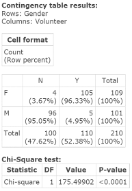
Figure 2. Contingency and chi‑square test table: Volunteer vs. Gender.
Guided Solution 1b
Copy the Contingency Table and Chi-Square Test Table into your Word file, ComputerLab6A.
- Create a new Word file called ComputerLab6B.
- Type the document title: ComputerLab6B.
- On the next line, type the heading: Contingency and Chi-Square Test Tables – Gender vs. Volunteers.
- On the next line, copy and paste the Contingency and Chi-Square Test Tables. For help with copying StatCrunch data, see Copying Materials from StatCrunch.
- Save your Word file, ComputerLab6B.
Task 2. Interpretation Question: Contingency and Chi‑Square Test Table: Gender vs. Volunteer
Copy the question below into your Word file ComputerLab6B, under the bottom item.
Interpret the two numbers displayed in the first cell of the Contingency table. Interpret the two numbers displayed in the cell in the first column/second row of the Contingency table.
Solution:
Use the contents of the Chi‑Square test table to conduct a test of hypothesis, at a 5% level of significance to determine whether the variables Gender and Volunteer are independent or related. Use the four-step P‑value Approach.
Solution:
Use the row percents displayed in the second column of the Contingency table to describe the relationship between the variables Gender and Volunteer.
Solution:
Based on your review of the pasted contingency and chi‑square test tables, type your answers in the solutions spaces provided. (If you need help answering these questions, see the Solutions that follow.) Save your Word file, ComputerLab6B.
Solution 2
The number 4 in the first cell of the Contingency table means that 4 of the 210 college staff surveyed are females who said No to engaging in volunteer activity.
The number in brackets in the first cell, 3.67%, means that 4 out of the 109 females surveyed (the row total) or 3.67% of the females surveyed, said No to engaging in volunteer activity.
In the cell in the first column/second row of the Contingency table, 96 males said No to engaging in volunteer activity, and 96/101 males or 95.05% of the males said No to engaging in volunteer activity.
Hypothesis test of independence: Four-step P‑value approach:
Step 1. HO: Gender and Volunteer are independent.
HA: Gender and Volunteer are related (dependent).Step 2. Test statistic = Chi‑Square = 175.49902 and related P‑value is less than 0.0001.
Step 3. As the P‑value is less than the level of significance of 0.05, reject HO.
Step 4. In the College Giving survey, there is a significant relationship between a staff member’s gender and his/her tendency to engage in volunteer activity.
- Based on the row percents in the second column of the Contingency table, while 96.33% of the females surveyed said Yes to engaging in volunteer activity, only 4.95% of the males said Yes to engaging in volunteer activity. In general, females tend to be significantly more engaged in volunteer activity than males.
Task 3. Verify the expected frequency assumption.
Verify the Expected Frequency Assumption made in conducting the Chi‑Square Test for Independence re the variables Gender and Volunteer in the College_Giving survey.
In using the Chi‑Square Test for Independence involving the variables Gender and Volunteer, you assumed that the expected frequency in each cell of the Contingency table is at least 5. The following Guided Solution illustrates how you can use StatCrunch to check this assumption.
Guided Solution 3a
Create a contingency table with expected frequencies.
- With the College_Giving data file open, click the menu option sequence Stat → Tables → Contingency → With Data, to display the Contingency table window.
- In the Row variable box, select Gender.
- In the Column variable box, select Volunteer.
- In the Display box, click Expected Count.
Click Compute to display the Contingency table with expected frequencies (counts), as in Figure 3.
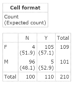
Figure 3. Contingency table with expected frequencies (counts).
Guided Solution 3b
Copy the contingency table and chi‑square test table into your Word file, ComputerLab6B.
- Open your Word file, ComputerLab6B.
- Below the bottom item, type the heading: Contingency Table with Expected Counts—Gender vs. Volunteers.
- On the next line, copy and paste the Contingency Table results. For help with copying StatCrunch data, see Copying Materials from StatCrunch.
- Save your Word file, ComputerLab6B.
Task 4. Interpretation Question: Contingency with Expected Counts Table: Gender vs. Volunteer
Copy the question below into your Word file ComputerLab6B, under the bottom item.
- Verify the Expected Frequency Assumption made in conducting the Chi‑Square Test for independence re the variables Gender and Volunteer in the College_Giving survey.
Based on your review of the pasted contingency table, type your answer in the solution space provided. (If you need help answering the question, see the Solution that follows.) Save your Word file, ComputerLab6B.
Solution 4
- The expected cell frequencies in the Contingency table are: 51.9, 57.1, 48.1, and 52.9. As each of these numbers exceeds an expected frequency of 5, the Expected Frequency Assumption made in the Chi‑Square Test for Independence is satisfied. You can have confidence in your conclusion that the variables Gender and Volunteer are significantly related.
Task 5. Exercise 13 Achievement and School Location, in Section 10.2 of your eText
A school district has randomly selected 317 elementary students to see if the location of the school – suburban vs. urban – is related to the students being successful in achieving basic skill levels in three subjects: math, reading, and science. The location and skill level achievement data for the 317 students are in the StatCrunch data file Ex10_2-13.txt, available in the Math 216 groups folder.
- Create a contingency table that cross-tabulates the student location and academic achievement in the different subjects, with Location as the row variable, and Subject as the column variable.
- Create a Chi‑Square Test Table that displays the test statistic and related P‑value that can be used to test whether the variables Location and Subject are independent or related.
Guided Solution 5a
Create a contingency and chi‑square test table involving the variables Location and Subject.
- Open the data file Ex10_2-13.txt from the Math 216 groups folder. (For help, see Accessing and Working in StatCrunch on the course home page.)
- Click the menu option sequence Stat → Tables → Contingency → With Data, to open the Contingency Table window.
- In the Row variable box, select Location.
- In the Column variable box, select Subject.
- In the Hypothesis tests box, click Chi‑Square test for independence.
Click Compute to display the contingency table and chi‑square test table, as in Figure 4.
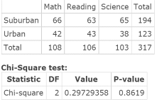
Figure 4. Contingency and Chi‑Square test table: Location vs. Subject.
Guided Solution 5b
Copy the Contingency Table and Chi-Square Test Table into your Word file, ComputerLab6B.
- Open your Word file, ComputerLab6B.
- Below the bottom item, type the heading: Contingency and Chi‑Square Test Tables–Location vs. Subject
- On the next line, copy and paste the Contingency and Chi-Square Test Tables. For help with copying StatCrunch data, see Copying Materials from StatCrunch.
- Save your Word file, ComputerLab6B.
Task 6. Interpretation Question: Contingency and Chi‑Square Test Table, Location vs. Subject.
Copy the question below into your Word file ComputerLab6B, under the bottom item.
Use the contents of the Chi-Square test table to conduct a test of hypothesis, at a 1% level of significance, to determine whether the variables Location and Subject are independent or related. Use the four-step P‑value approach.
Solution:
Based on your review of the pasted contingency and chi‑square test tables, type your answer in the solution space provided. (If you need help answering the question, see the Solution that follows.) Save your Word file, ComputerLab6B.
Solution 6
Hypothesis Test of Independence: Four‑step P‑value Approach:
Step 1. HO: Location and Subject are independent.
HA: Location and Subject are related (dependent).Step 2. Test statistic = Chi-Square = 0.29729358 and related P‑value is 0.8619.
Step 3. As the P‑value exceeds the level of significance of 0.01, do not reject HO.
Step 4. The two variables are independent. There appears to be no relationship between the school location and the level of student achievement in the three subjects math, reading, and science.
Task 7. Verify the expected frequency assumption.
Verify the Expected Frequency Assumption made in conducting the Chi‑Square Test for Independence re the variables Location and Subject in the Ex10_2-13.txt data file.
In using the Chi-Square Test for Independence involving the variables Location and Subject, you assumed that the expected frequency in each cell of the contingency table is at least 5. The following Guided Solution illustrates how to use StatCrunch to check this assumption.
Guided Solution 7a
Create a contingency table with expected frequencies.
- With the Ex10_2-13.txt data file open in StatCrunch, click the menu option sequence Stat → Tables → Contingency → With Data, to display the Contingency Table window.
- In the Row variable box, select Location.
- In the Column variable box, select Subject.
- In the Display box, click Expected Count.
Click Compute to display the Contingency table with expected frequencies (counts), as in Figure 5.
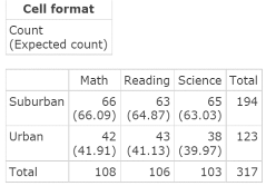
Figure 5. Contingency table with expected frequencies (counts).
Guided Solution 7b
Copy the Contingency table with expected counts into your Word file, ComputerLab6B.
- Open your Word file, ComputerLab6B.
- Below the bottom item, type the heading: Contingency Table with Expected Counts–Location vs. Subject.
- On the next line, copy and paste the Contingency table. For help with copying StatCrunch data, see Copying Materials from StatCrunch.
- Save your Word file, ComputerLab6B.
Task 8. Interpretation Question: Contingency with Expected Counts Table: Location vs. Subject
Copy the question below into your Word file ComputerLab6B, under the bottom item.
Verify the Expected Frequency Assumption made in conducting the Chi‑Square Test for Independence re the variables Location and Subject related to the Ex10_2-13.txt data file.
Solution:
Based on your review of the contingency table, type your answer in the solution space provided. (If you need help answering the question, see the Solution that follows.) Save your Word file, ComputerLab6B.
Solution 8
- Each of the expected cell frequencies in the Contingency table with counts exceeds the expected frequency of 5. The Expected Frequency Assumption made in the Chi‑Square Test for Independence is satisfied. You can have confidence in your conclusion that the variables Location and Subject are independent.
Activity 2. One way Analysis of Variance (ANOVA)
In this activity, you will conduct tests of hypotheses that involve comparing the means of more than two populations.
Task 9. Exercise 9 from Elementary Statistics, 6th edition
Exercise 9. Ages of Professional Athletes
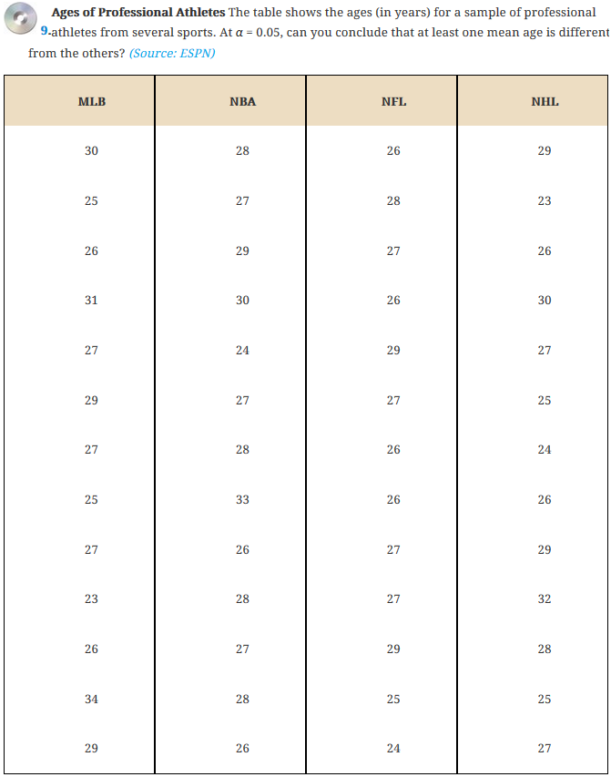
The eText StatCrunch data file Ex10_4-9.txt, located in the AU Math 216 group folder, displays the ages of 13 randomly selected players from each of four major sports leagues: MLB, NBA, NFL, and NHL. Use StatCrunch to do the following:
- Conduct an ANOVA to see if at least one mean age (in one sports league) is different from the other leagues, at a 5% level of significance.
- Test the assumption of equal variances at a 5% level of significance.
- Test the assumption of normality at a 5% level of significance.
Guided Solution 9a
Conduct an ANOVA to see if at least one mean age (in one sports league) is different from the other leagues, at a 5% level of significance. (Conduct an ANOVA comparing the mean ages of four sports leagues.)
| Step 1. | Specify the hypotheses: HO: μ1 = μ2 = μ3 = μ4 |
| Step 2. | Use StatCrunch to compute the appropriate test statistic and related P‑value. |
Guided Solution 9b
Compute the test statistic and related P‑value. (Step 2)
- Open the eText data file Ex10_4-9.txt located in the Math 215 group folder at the StatCrunch website.
- Click the menu sequence Stat → ANOVA → One Way, to display the One way ANOVA window.
- In the Selected Columns box, select all four variables (use the Ctrl key).
- Under Options, select Test homogeneity of variance and Levene’s test.
Click Compute to display the Analysis of Variance results window, as in Figure 6. As the ANOVA table indicates, the test statistic = F-Stat = −0.61502347; related P‑value = 0.6086.
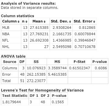
Figure 6. ANOVA results window.
| Step 3. | As the P‑value = 0.6086 exceeds alpha = 0.05, do not reject HO. |
| Step 4. | You cannot conclude that the mean ages differ between the four sports leagues. |
Guided Solution 9c
Copy the ANOVA results window into your Word file, ComputerLab6B.
- Open your Word file, ComputerLab6B.
- Below the bottom item, type the heading: ANOVA results window Section 10.4 Exercise 9.
- On the next line, copy and paste the ANOVA results window. For help with copying StatCrunch data, see Copying Materials from StatCrunch.
- Save your Word file, ComputerLab6B.
Task 10. Interpretation Questions: ANOVA Hypothesis Test: Comparing Population Mean Ages Between Sports Leagues
Copy the question below into your Word file ComputerLab6B, under the bottom item.
Use the contents of the ANOVA table to conduct a test of hypothesis, at a 5% level of significance, to determine whether the mean population age differs between the four major sports leagues.
Solution: (4 step P‑value Approach)
Based on your review of the ANOVA table, type your answer in the solution space provided. (If you need help answering the question, see the Solution that follows.) Save your Word file, ComputerLab6B.
Solution 10
ANOVA Hypothesis Test: Four‑step P‑value approach:
Step 1. HO: μ1 = μ2 = μ3 = μ4
HA: At least one league’s population mean age differs from other leagues’ mean ages.Step 2. The test statistic = F‑Stat = 0.61502347; related P‑value = 0.6086.
Step 3. As the P‑value exceeds the level of significance of 0.05, do not Reject HO.
Step 4. You cannot conclude that the mean ages differ between the 4 different sports leagues.
Task 11. Interpretation Question: Test the assumption using Levene’s Test for Homogeneity of Variances.
In conducting the ANOVA Test of Hypothesis, you assumed that each of the four samples come from populations with equal variances. Test the assumption that all four samples come from populations of equal variances at a 5% level. Use an equal variances test called Levene’s Test for Homogeneity of Variances.
Above, you used StatCrunch to conduct Levene’s Test for Homogeneity of Variances. Test the assumption of normality at a 5% level of significance.
Type the four-step P‑value approach for hypothesis tests and the question below into your ComputerLab6B Word file, below the bottom item. (If you need help answering the question, see the Solution that follows.)
Solution 11
| Step 1. | HO: σ12 = σ22 = σ32 = σ42 |
| Step 2. | The test statistic and related P‑value. |
| Step 3. | As the P‑value exceeds the level of significance of 0.05, do not Reject HO. |
| Step 4. | You can conclude that the assumption of equal variances is reasonable. |
Task 12. Use the Shapiro-Wilk Test for Normality to determine if each of the four samples in the data file Ex10_4‑9 appears to come from normal populations.
In conducting the ANOVA Test of Hypothesis, you assumed that each of the four samples comes from a normal population. Here, you will check the validity of this assumption.
Use the Shapiro-Wilk Test for Normality to determine if each of the four samples in the data file Ex10_4-9 appears to come from a normal population. Assume a 5% level of significance for this test.
| Step 1. | HO: Each population is normally distributed. |
| Step 2. | Use StatCrunch to compute the Shapiro‑Wilk test statistic and related P‑value. |
Guided Solution 12
Use StatCrunch to Compute the Shapiro-Wilk test statistic and P‑value. (Step 2)
- With the data file Ex10_4-9.txt open, click the menu sequence Stat → Goodness-of-fit → Normality Test, to display the Normality test window.
- In the Select columns box, select all four variables (use the Ctrl key).
- In the Test box, select Shapiro‑Wilk.
Click Compute to display the Shapiro‑Wilk Results window, as shown in Figure 7. The P‑values for the four samples are: 0.722, 0.278, 0.4625, 0.9754.
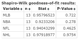
Figure 7. Shapiro‑Wilk results window.
| Step 3. | As each of the P‑values exceeds alpha = 0.05, do not reject HO. |
| Step 4. | You cannot conclude that the population is not normally distributed (therefore, the assumption of normal population is reasonable) for each of the four samples. |
As you have verified the validity of both the normality and equal variances assumption, you can have confidence in the ANOVA test conclusion that you cannot conclude that the mean ages differ between the four different sports leagues.
Task 13. Try It Yourself 1 from Elementary Statistics, 6th edition
The StatCrunch data file Ex10_4-TIY1.txt, available in the Math 216 group folder, shows a company’s monthly sales in four sales regions: North, East, South, and West.
Use StatCrunch to conduct an ANOVA Hypothesis Test to determine if the mean monthly sales differs between the four sales regions, at a 5% level of significance.
Guided Solution 13a
Use StatCrunch to display the appropriate ANOVA results window. It can be used to conduct the desired ANOVA Test of Hypothesis and to test the Equal Variance Assumption. Test the assumption of normality at a 5% level of significance.
Display ANOVA Results Window: Section 10.4 Try It Yourself 1
- Open the data file Ex10_4-TIY1.txt available in the Math 216 group folder. (For help, see Accessing and Working in StatCrunch on the course home page.)
- Click the menu sequence Stat → ANOVA → One Way, to display the One Way ANOVA window.
- In the Select columns box, select all four variables (use the Ctrl key).
- Under Option, select Test homogeneity of variance and Levene’s test.
Click Compute to display the Analysis of Variance results window, as in Figure 8.
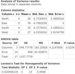
Figure 8. ANOVA results window: Section 10.4 Try It Yourself 1
Guided Solution 13b
Copy the ANOVA results window into your Word file, ComputerLab6B.
- Open your Word file, ComputerLab6B.
- Below the bottom item, type the heading: ANOVA results window: Section 10.4 Try It Yourself 1.
- On the next line, copy and paste the ANOVA results window. (For help with copying StatCrunch data, see Copying Materials from StatCrunch.)
- Save your Word file, ComputerLab6B.
Task 14. Interpretation Questions: ANOVA Hypothesis Test: Comparing Population Mean Sales Between Regions
Copy the question below into your Word file ComputerLab6B, under the bottom item.
Use the contents of the ANOVA Table to conduct a test of hypothesis, at a 5% level of significance, to determine whether the mean monthly sales differ between the four sales regions.
Solution: (four‑step P‑value approach)
Use the contents of the ANOVA results window to test the equal variances assumption.
Solution: (four‑step P‑value approach)
Based on your review of the ANOVA table, type your answers in the solutions spaces provided. (If you need help answering these questions, see the Solutions section that follows them.) Save your Word file, ComputerLab6B.
Solution 14
ANOVA Hypothesis Test: Four-step P‑value approach:
Step 1. HO: μ1 = μ2 = μ3 = μ4
HA: At least one region’s mean monthly sales differ from other regions’ mean monthly sales.Step 2. The ANOVA Table in the ANOVA results window shows the test statistic = F‑Stat = 4.2197856; related P‑value = 0.0254.
Step 3. As the P‑value is less than the level of significance of 0.05, reject HO.
Step 4. You can conclude that there is a difference in the mean monthly sales among the different sales regions at a 5% level of significance.
In conducting the ANOVA Test of Hypothesis, you assumed that the four samples come from populations with equal variances. Here, you will use StatCrunch to conduct Levene’s Test for Homogeneity of Variances.
Step 1. HO: σ12 = σ22 = σ322 = σ42.
HA: At least one pair of population variances differs.Step 2. The test statistic and related P‑value:
If you review the bottom section of the ANOVA results window Levene’s Test for Homogeneity (as displayed in Figure 8) you will see that the test statistic = 0.020456134 and the P‑value = 0.9958.Step 3. As the P‑value exceeds the level of significance of 0.05, do Not Reject HO.
Step 4. You can conclude that the assumption of equal variances is reasonable.
Task 15. Test the assumption of normality.
In conducting the ANOVA Test of Hypothesis, you assumed that the four samples come from normal populations. Here, you will check the validity of this assumption.
Test the assumption of normality at a 5% level of significance. Use the Shapiro‑Wilk Test for Normality to determine if each of the four samples in the data file Ex10_4-TIY1 appears to come from a normal population. Assume a 5% level of significance for this test.
| Step 1. | HO: Each population is normally distributed. |
| Step 2. | Use StatCrunch to compute the Shapiro‑Wilk test statistic and related P‑value. |
Guided Solution 15
Using StatCrunch to Compute the Shapiro-Wilk test statistic and P‑value. (Step 2)
- With the data file Ex10_4-TIY1.txt open, click the menu sequence Stat → Goodness-of-fit → Normality Test.
- In the Select columns box, select all four variables (use the Ctrl key).
- In the Test box, select Shapiro‑Wilk.
Click Compute to display the Shapiro‑Wilk results window, as shown in Figure 9. The P‑values for the four samples are 0.9999, 0.8902, 0.1116, 0.3744.
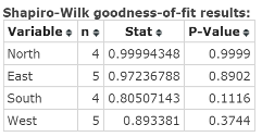
Figure 9. Shapiro-Wilk results window.
| Step 3. | Make a decision based on comparing the P‑value with the level of significance, alpha, as follows: Since each of the four P‑values exceeds alpha = 0.05, do not reject HO. |
| Step 4. | You cannot conclude that the population is not normally distributed (therefore, the assumption of normal population is reasonable) for each of the four samples. |
As you have now verified the validity of both the normality and equal variances assumption, you can have confidence in the ANOVA Test conclusion that there is a difference in the mean monthly sales among the different sales regions at a 5% level of significance.
