Mathematics 216 Computer-oriented Approach to Statistics

Computer Lab 3B
with Guided Solutions (Technology Manual)

Here, you will use StatCrunch to compute normal distribution probabilities.

Task 1. Exercise 11 from Elementary Statistics, 6th edition

Exercise 11. Utility Bills

Guided Solution 1a

For (a) is less than $70:

Because the normal variable is a continuous variable, P(X < 70) = P(X ≤ 70)

P(X is less than $70) = P(X < 70) = P(X ≤ 70)

Normal Probability: P(X ≤ 70)

1. Open a new data table in StatCrunch.
2. Click the menu sequence: Stat → Calculators → Normal. This will display a normal probabilities window containing the graph of the normal distribution.
3. Near the top of the graph window, click the Standard button.
4. In the text boxes below the graph of the normal distribution:
   1. In the Mean box, type 100.
   2. In the Std. Dev. box, type 12.
   3. In the P(X) box , select ≤ in the first box, and type in 70 in the second box.

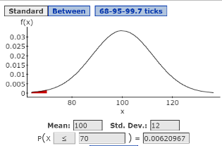
5. Click Compute to display the solution P(X ≤ 70) = .00620967. See Figure 1.

   

   Figure 1. Normal Probability Window: P(X ≤ 70)

Guided Solution 1b

Copy the normal probability distribution graph into a new Word file called ComputerLab3B.

1. Create a new Word file entitled ComputerLab3B.
2. Type its title, ComputerLab3B.
3. Below the title, type: Normal Probabilities P(X < 70) = P(X ≤ 70.
4. Below that, copy and paste the normal probability distribution window that you just created. (For help with copying StatCrunch data, see Copying Materials from StatCrunch.)
5. Save the Word file, ComputerLab3B.

Guided Solution 1c

For (b) is between $90 and $120

P(X is between $90 and $120)

Normal Probability: P(X is between $90 and $120)

1. With a new data file open in StatCrunch, click the menu sequence: Stat → Calculators → Normal.
2. Near the top of the graph window, click the Between button.
3. In the text boxes below the graph:
   1. In the Mean box, type 100.
   2. In the Std. Dev. box, type 12.
   3. In the P(X) box , type 90 in the first box ,and type in 120 in the second box.
4. Click Compute to display the solution P(X is between 90 and 120 inclusive) = 0.74988127.

Guided Solution 1d

1. Copy the graph window into your Word file, ComputerLab3B. Follow the steps in Guided Solution 1b, but type the title Normal Probabilities P(X is between 90 and 120 inclusive).

Guided Solution 1e

For (c) is more than $140:

Because the normal variable is a continuous variable, P(X > 140) = P(X ≥ 140)

P(X more than $140) = P(X > 140) = P(X ≥ 140)

Normal Probability: P(X ≥ 140)

1. With a new data file open in StatCrunch, click the menu sequence: Stat → Calculators → Normal.
2. Near the top of the graph window, click the Standard button.
3. In the text boxes below the graph:
   1. In the Mean box, type 100.
   2. In the Std. Dev. box, type 12.
   3. In the P(X) box , select  ≥ in the first box and type 140 in the second box.
4. Click Compute to display the solution P(X ≥ 140) = .00042906.

Guided Solution 1f

1. Copy the graph window into your Word file, ComputerLab3B. Follow the steps in Guided Solution 1b, but type the title Normal Probabilities P(X > 140) = P(X ≥ 140).

Here, you will be given probabilities or percentages related to a normal distribution and you will be asked to find the corresponding X value(s). This type of problem is often called an Inverse Normal problem.

Task 2. Exercise 33 from Elementary Statistics, 6th edition

Exercise 33. Heart Transplant Waiting Times

The number of days spent waiting for a heart transplant by people aged 35‑49 is approximated by a normal distribution with a mean of 203 days and a standard deviation of 25.7 days.

Guided Solution 2a

(a) What waiting time represents the 5th percentile?

To use StatCrunch  to compute the solution to this question, you need to restate the problem in this way: Find the value of X such that P(X ≤ value?) = 0.05.

Normal Distribution: P(X ≤ value?) = 0.05

1. With a new data file open in StatCrunch, click the menu sequence: Stat → Calculators → Normal.
2. Near the top of the graph window, click the Standard button.
3. In the text boxes below the graph:
   1. In the Mean box, type 203.
   2. In the Std. Dev. box, type 25.7.

   3. In the P(X) box , select ≤ in the first box, leave the second box blank, and type 0.05 in the third box. See Figure 2.

      

      Figure 2. Inverse Normal Probability Window: P(X ≤ value?) = 0.05

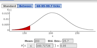
4. Click Compute to display  P(X ≤ 160.7272) = .05; here, the solution is X = 160.7272. The appropriate area under the normal curve is now displayed, as shown in Figure 3. The conclusion is that 160.7272 days is the waiting time that represents the 5th percentile. In other words, 5% of the waiting times tend to be less than or equal to 160.7272 days, and 95% of the waiting times tend to be more than 160.7272 days.

   

   Figure 3. Normal probability window with graph displayed

Guided Solution 2b

1. Copy the graph window into your Word file, ComputerLab3B. Follow the steps in Guided Solution 1b, but type the title Inverse Normal Problem Normal Probabilities P(X ≤ 160.7272) = 0.05.

Guided Solution 2c

(b) What waiting time represents the 3rd quartile?

To use StatCrunch to compute the solution to this question, you need to restate the problem like this: Find the value of X such that P(X ≤ value?) = 0.75

Normal Distribution: P(X ≤ value?) = 0.75

1. With a new data file open in StatCrunch, click the menu sequence: Stat → Calculators → Normal.
2. Near the top of the graph window, click the Standard button.
3. In the text boxes below the graph:
   1. In the Mean box, type 203.
   2. In the Std. Dev. box, type 25.7.
   3. In the P(X) box , select ≤ in the first box, leave the second box blank, and type 0.75 in the third box.
4. Click Compute to display P(X ≤ 220.33439) = .75; here the solution is X = 220.33439. The conclusion is that 220.33439 days is the waiting time that represents the 75th percentile. In other words, 75% of waiting times tend to be less than or equal to 220.33439 days, and 25% of the waiting times tend to be more than 220.33439 days.

Guided Solution 2d

1. Copy the graph window into your Word file, ComputerLab3B. Follow the steps in Guided Solution 1b, but type the title Inverse Normal Problem Normal Probabilities P(X ≤ 220.33439) = 0.75.