Mathematics 216 Computer-oriented Approach to Statistics
Computer Lab 6A
with Guided Solutions (Technology Manual)
With the aid of the Guided Solutions, you will use StatCrunch to work through each of the following Activities, which relate to the eText’s Chapter 9 Correlation and Regression.
Activity 1. Conduct a correlation analysis.
In Activity 1, you will:
- Create a Scatter plot with a country’s GDP on the X axis and CO2 Emissions on the Y axis.
- Compute the correlation coefficient, r, to measure the strength of the linear relationship between GDP and CO2 emissions.
- At a 5% level of significance, use the t‑test to see if the population correlation coefficient, ρ, is significantly different from zero.
Task 1. Example 1 from Elementary Statistics, 6th edition
Example 1 Correlation Between GDP and CO2
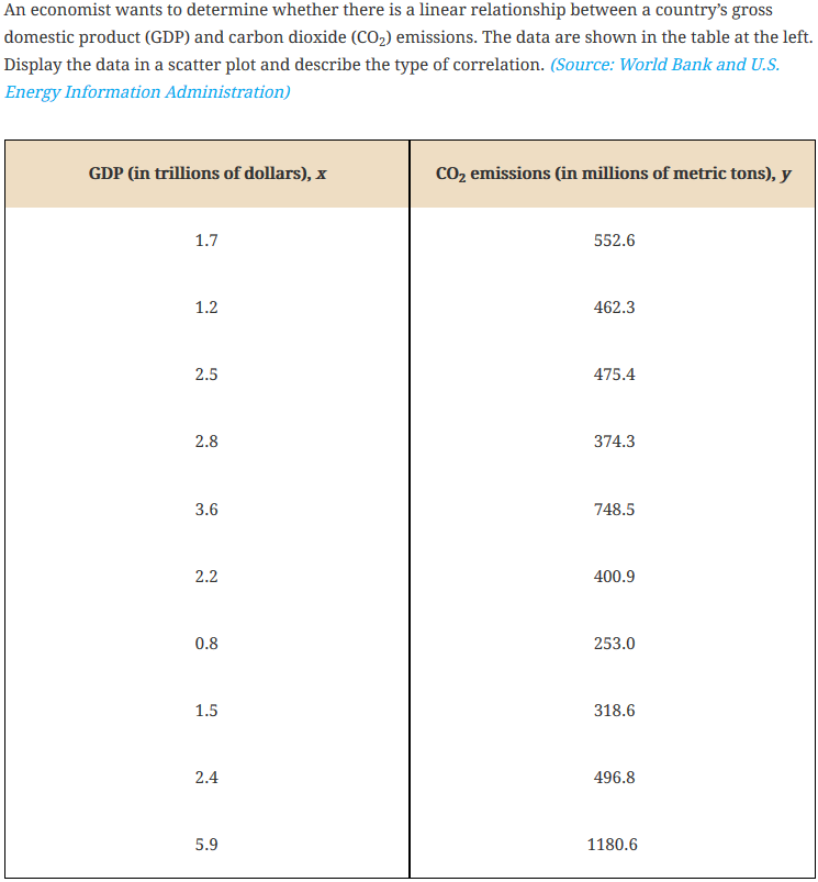
A random sample of 10 pairs of GDP and CO2 values (for 10 different countries) is shown in the StatCrunch data file Countries.txt, available in the StatCrunch Math 216 groups folder.
Guided Solution 1a
Construct a Scatter plot for the two variables GDP (X variable) and CO2 (Y variable) emissions.
- Open the StatCrunch data file Countries.txt. (See Open a Groups Data File in StatCrunch in Accessing and Working in StatCrunch on the course home page if you need help.)
- Click the menu sequence Graph → Scatter Plot, to display a Scatter Plot window.
- In the X variable box, select the GDP variable.
- In the Y variable box, select the CO2 variable.
Click Compute to display the Scatter plot, as shown in Figure 1.
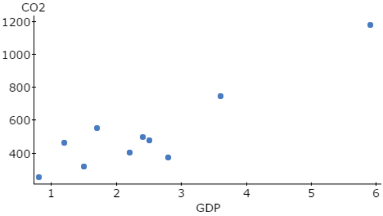
Figure 1. Scatter plot: GDP vs. CO2 emissions.
Guided Solution 1b
Copy the Scatter plot into your Word file, ComputerLab6A.
- Create a new Word file called ComputerLab6A.
- Type the document title: ComputerLab6A.
- Below the title, type the heading: Scatter plot of GDP vs. CO2 Emissions.
- On the next line, copy and paste the Scatter plot you created. (For help with copying StatCrunch data, see Copying Materials from StatCrunch.)
- Save your Word file, ComputerLab6A.
Task 2. Interpretation Question: Scatter plot of GDP vs. CO2 Emissions
Copy the question below into your Word file ComputerLab6A, under the bottom item.
Based on the Scatter plot you created, would you suggest that GDP and CO2 emissions are positively or negatively correlated? Briefly explain.
Solution:
Based on your review of the graph, type your answer in the solution space provided. (If you need help answering the question, see the Solution that follows.) Save your Word file, ComputerLab6A.
Solution 2
- Positively correlated, because higher levels of GDP are associated with higher levels of CO2 emissions.
Task 3. Compute the correlation coefficient, r, to measure the strength of the linear relationship between GDP and CO2 emissions.
Guided Solution 3a
Compute the correlation coefficient, r.
- With the data file Countries.txt open, click the menu sequence Stat → Summary Stats → Correlation, to display a Correlation window.
- Select both variables, GDP and CO2. (Use the Ctrl key.)
Click Compute to display the correlation coefficient as: 0.91159239. See Figure 2.

Figure 2. Correlation coefficient output.
Guided Solution 3b
Copy the Correlation output into your Word file, ComputerLab6A.
- Open your Word file, ComputerLab6A.
- Below the bottom item, type the title: Correlation Coefficient.
- Below the title, type the heading: Scatter plot of GDP vs. CO2 Emissions.
- On the next line, copy and paste the Scatter plot you created. (For help with copying StatCrunch data, see Copying Materials from StatCrunch.)
- Save your Word file, ComputerLab6A.
Task 4. Interpretation Question: Correlation Coefficient
Copy the question below into your Word file ComputerLab6A, under the bottom item.
What does a correlation coefficient equal to 0.91159239 mean in terms of the relationship between GDP and CO2 emissions?
Solution:
Based on your review of the Correlation output, type your answer in the solution space provided. (If you need help answering the question, see the Solution that follows.) Save your Word file, ComputerLab6A.
Solution 4
- A correlation coefficient equal to 0.91159239 means that there is a strong positive linear relation between GDP and CO2 emissions.
Task 5. T‑test to see if the population correlation coefficient, ρ, is significantly different from zero.
At a 5% level of significance use the t‑test to see if the population correlation coefficient, ρ, is significantly different from zero. Use the four‑step P‑value Approach
| Step 1. | HO: The population correlation coefficient ρ = 0. |
| Step 2. | Use StatCrunch to compute the test statistic and related P-value. |
Guided Solution 5a
Compute the related P‑value. (Step 2)
- With the data file Countries.txt (available in the StatCrunch Math 216 groups folder) open, click the menu sequence Stat → Summary Stats → Correlation, to display the Correlation window.
- Select both variables, GDP and CO2, using the Ctrl key.
- In the Display section, select Two-sided P‑value.
Click Compute to display the Correlation coefficient and the related P‑value, as in Figure 3. The Correlation coefficient = 0.91159239 and the P‑value = 0.0002.

Figure 3. Correlation coefficient and related P‑value.
| Step 3. | As the P-value = 0.0002 is less than alpha = 0.05, reject HO. |
| Step 4. | A country’s GDP level is significantly correlated with the country’s CO2 emission levels |
Guided Solution 5b
Copy the correlation output into your Word file, ComputerLab6A.
- Open your Word file ComputerLab6A.
- Below the bottom item, type the heading: Correlation Coefficient and P‑value.
- On the next line, type the subheading: Correlation Coefficient.
- On the next line, copy and paste the Correlation output you created. For help with copying StatCrunch data, see Copying Materials from StatCrunch.
- Save your Word file, ComputerLab6A.
Task 6. Interpretation Question: Hypothesis test re significance of correlation coefficient
In your Word file ComputerLab6A, under the bottom item type/paste the four-steps (P‑value approach) to test the hypothesis related to the significance of the population correlation coefficient. (If you need help, see the Solution that follows.) Save your Word file, ComputerLab6A.
Solution 6
| Step 1. | HO: The population correlation coefficient ρ = 0. |
| Step 2. | Related P‑value = 0.0002. |
| Step 3. | As the P‑value = 0.0002 is less than alpha = 0.05, reject HO. |
| Step 4. | A country’s GDP level is significantly correlated with the country’s CO2 emission. |
Task 7. Exercise 21 from Elementary Statistics, 6th edition
Exercise 21. Age and Blood Pressure

The ages (in years) of ten men and their systolic blood pressures (in millimeters of mercury) are displayed in the data file Ex9_1-21.txt located in the Math 216 group folder at the StatCrunch website. Use StatCrunch to:
- Create a Scatter plot with Age on the X axis and Systolic blood pressure on the Y axis.
- Compute the Correlation coefficient, r, to measure the strength of the linear relationship between Age and Systolic blood pressure.
- At a 5% level of significance, use the t‑test to see if the population correlation coefficient, ρ, is significantly different from zero.
Guided Solution 7a
Construct a Scatter plot for the two variables. Age (X) and Systolic blood pressure (Y).
- Open the data file Ex9_1-21.txt. (For help, see Accessing and Working in StatCrunch on the course home page.)
- Click the menu sequence Graph → Scatter Plot, to display the Scatter Plot window.
- In the X variable box, select the Age variable.
- In the Y variable box, select the Systolic blood pressure variable.
Click Compute to display the Scatter plot, as in Figure 4.
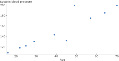
Figure 4. Scatter plot: Age vs. Systolic blood pressure.
Guided Solution 7b
Copy the Scatter plot into your Word file, ComputerLab6A.
- Open your Word file ComputerLab6A.
- Below the bottom item, type the heading: Scatter plot: Age vs. Systolic blood pressure.
- On the next line, copy and paste the Scatter plot you created. For help with copying StatCrunch data, see Copying Materials from StatCrunch.
- Save your Word file, ComputerLab6A.
Task 8. Interpretation Question: Scatter plot of Age vs. Systolic blood pressure.
Copy the question below into your Word file ComputerLab6A, under the bottom item.
Based on the Scatter plot just pasted, would you suggest that Age and Systolic blood pressure are positively or negatively correlated? Briefly explain.
Solution:
Based on your review of the Scatter plot, type your answer in the solution space provided. (If you need help answering the question, see the Solution that follows.) Save your Word file, ComputerLab6A.
Solution 8
- Positively correlated, because higher levels of Age are associated with higher levels of Systolic blood pressure.
Task 9. Compute the Correlation Coefficient, r.
Guided Solution 9a
Compute the Correlation Coefficient, r, to measure the strength of the linear relationship between Age and Systolic blood pressure.
- With the data file Ex9_1-21.txt open, click the menu sequence Stat → Summary Stats → Correlation, to display the Correlation window.
- In the Select columns box, select both variables, Age and Systolic blood pressure, using the Ctrl key.
Click Compute to display the correlation coefficient as 0.90838623. See Figure 5.

Figure 5. Correlation coefficient output.
Guided Solution 9b
Copy the Correlation Coefficient Output into your Word file, ComputerLab6A.
- Open your Word file ComputerLab6A.
- Below the bottom item, type the heading: Correlation Coefficient.
- On the next line, copy and paste the Correlation Coefficient Output you created. For help with copying StatCrunch data, see Copying Materials from StatCrunch.
- Save your Word file, ComputerLab6A.
Task 10. Interpretation Question: Correlation Coefficient
Copy the question below into your Word file ComputerLab6A, under the bottom item.
What does a correlation coefficient equal to 0.90838623 mean in terms of the relationship between Age and Systolic blood pressure?
Solution:
Based on your review of the Correlation output, type your answer in the solution space provided. (If you need help answering the question, see the Solution that follows.) Save your Word file, ComputerLab6A.
Solution 10
- A correlation coefficient equal to 0.90838623 means that there is a strong positive linear relation between Age and Systolic blood pressure.
Task 11. Use the t‑test to see if the population correlation coefficient, ρ, is significantly different from zero.
At a 5% level of significance, use the t‑test to see if the population correlation coefficient, ρ, is significantly different from zero. Use the four‑step P‑value approach.
| Step 1. | HO: The population correlation coefficient ρ = 0. |
| Step 2. | Use StatCrunch to compute the test statistic and related P‑value. |
Guided Solution 11a
Compute the related P‑value. (Step 2)
- With the data file Ex9_1-21.txt open, click the menu sequence Stat → Summary Stats → Correlation, to display the Correlation window.
- In the Select columns box, select both variables, Age and Systolic blood pressure, using the Ctrl key.
- In the Display section, select Two-sided P‑value.
Click Compute to display the Correlation Coefficient along with the related P‑value, as in Figure 6. The Correlation coefficient = 0.90838623 and the P‑value = 0.0003.

Figure 6. Correlation coefficient and related P‑value.
| Step 3. | As the P‑value = 0.0003 is less than alpha = 0.05, reject HO. |
| Step 4. | Age is significantly correlated with Systolic blood pressure. |
Guided Solution 11b
Copy the Correlation Output into your Word file, ComputerLab6A.
- Open your Word file ComputerLab6A.
- Below the bottom item, type the heading: Correlation Coefficient and related P‑value.
- On the next line, copy and paste the Correlation Output you created. For help with copying StatCrunch data, see Copying Materials from StatCrunch.
- Save your Word file, ComputerLab6A.
Task 12. Interpretation Question: Hypothesis Test re Significance of Correlation Coefficient
Below the bottom item in your Word file ComputerLab6A, type/paste the four steps (P‑value approach) used to test the hypothesis related to the significance of the population correlation coefficient. (If you need help answering the question, see the Solution that follows.) Save your Word file, ComputerLab6A.
Solution 12
| Step 1. | HO: The population correlation coefficient ρ = 0. |
| Step 2. | Related P‑value = = 0.0003. |
| Step 3. | As the P‑value = 0.0003 is less than alpha = 0.05, reject HO. |
| Step 4. | Age is significantly correlated with Systolic blood pressure. |
Activity 2. Conduct Linear Regression Analysis
Here, you will apply regression analysis on the paired (GDP, CO2 emissions) sample data in the data file Countries.txt. Specifically, your task is to formulate a linear regression equation that will predict CO2 emissions (Y) based on given levels of GDP (X). Note that, in the StatCrunch data file, GDP values are in trillions of dollars and CO2 Emissions are in millions of metric tons.
Task 13. Example 1 from Elementary Statistics, 6th edition
Example 1 Correlation Between GDP and CO2

In this task, you want to determine whether there is a significant linear equation relating a country’s GDP (X) and CO2 emissions (Y). A random sample of 10 pairs of GDP and CO2 values (for 10 different countries) is in the data file Countries.txt, available in the StatCrunch Math 216 groups folder. Using this data, do the following:
- Find the equation of the linear regression line with GDP being the independent variable.
- Plot the regression line along with the Scatter plot.
- Compute the Coefficient of Determination, r squared.
- Test to see if the slope of the regression line significantly exceeds zero.
- Construct a 95% prediction interval for CO2 Emissions when a country’s GDP level is 3.5 trillion dollars.
Guided Solution 13a
Find the equation of the linear regression line. Plot the regression line along with the Scatter plot (called the Fitted plot)
- Open the data file Countries.txt. (See Open a Groups Data File in StatCrunch in Accessing and Working in StatCrunch on the course home page if you need help.)
- Click the menu sequence Stat → Regression → Simple Linear, to display the Simple Linear Regression window.
- In the X variable box, select GDP.
- In the Y variable box, select CO2.
- In Graphs section, select Fitted Line Plot.
Click Compute to display the Simple linear regression results window, as in Figure 7.
As the Simple Linear Regression window indicates, the equation of the regression line is: CO2 = 115.72492 + 166.90044 GDP, showing that the Regression Line has a Y intercept of 115.72492 and a slope of 166.90044.
Note that you could formulate this equation a) directly from the third line of the Simple linear regression results window, or b) from the Estimate column of the Parameter estimates table.
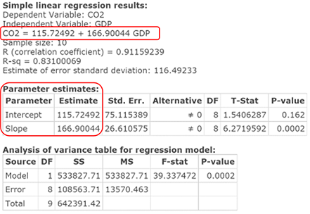
Figure 7. Simple Linear Results window—first screen.
Guided Solution 13b
Copy the Regression output into your Word file, ComputerLab6A.
- Open your Word file ComputerLab6A.
- Below the bottom item, type the heading: Regression Equation.
- On the next line, copy and paste the Regression output you created. For help with copying StatCrunch data, see Copying Materials from StatCrunch.
- Save your Word file, ComputerLab6A.
Guided Solution 13c
Plot of regression line fitted to the scatter plot.
With the first screen of the Simple linear regression results window displayed, click the right arrow button (at the bottom right of the window). A second screen will display, showing the plot of the regression line fitted to the scatter plot, as in Figure 8.
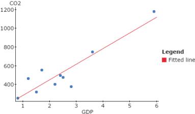
Figure 8. Plot of fitted regression line.
Note that the ten blue points represent the ten paired (GDP, CO2) sample values in the Countries.txt data file, while the upward sloping red line represents the Regression line corresponding to the regression equation: CO2 = 115.72492 + 166.90044 GDP. The Y intercept and slope of the Regression Line are 115.72492 and 166.90044 respectively.
Guided Solution 13d
Copy the Plot of Regression Line Fitted to the Scatter plot into your Word file, ComputerLab6A.
- Open your Word file ComputerLab6A.
- Below the bottom item, type the heading: Plot of Regression Line Fitted to the Scatter plot.
- On the next line, copy and paste the graph you created. For help with copying StatCrunch data, see Copying Materials from StatCrunch.
- Save your Word file, ComputerLab6A.
Task 14. Interpretation Questions: Regression Equation and Fitted Line Plot
Copy the questions below into your Word file ComputerLab6A, under the bottom item.
What is the slope coefficient of the regression equation and what does it suggest about the relation between GDP and CO2 Emissions?
Solution:
How does the slope coefficient relate to the plotted Regression line?
Solution:
Interpret the upward sloping nature of the Regression line.
Solution:
Based on your review of the Regression output, type your answers in the solution spaces provided. (If you need help answering the questions, see the Solution section that follows.) Save your Word file, ComputerLab6A.
Solution 14
- The slope coefficient is 166.90044, which indicates that for every 1 trillion dollar increase in GDP, the CO2 emissions increase by 166.90044 million metric tons of emissions.
- The slope coefficient of 166.90044 measures the slope of the Regression line.
- The upward sloping nature of the Regression line suggests a positive linear relation between GDP and CO2 emissions.
Task 15. Find the Coefficient of Determination, r squared.
Guided Solution 15
Coefficient of Determination, r squared.
- With the first screen of the Simple linear regression results window displayed, locate the output called R-sq = 0.83100069. This is the Coefficient of Determination. It is the same as the Correlation Coefficient squared.
Task 16. Interpretation Questions: Coefficient of Determination, r squared
Copy the questions below into your Word file ComputerLab6A, under the bottom item.
What does the Coefficient of determination suggest about the relation between GDP and CO2 emissions?
Solution:
What does the Coefficient of determination measure in terms of the plot of the fitted regression line?
Solution:
Based on your review of the Regression output, type your answers in the solutions spaces provided. (If you need help answering these questions, see the Solutions that follow.) Save your Word file, ComputerLab6A.
Solution 16
- R-sq = 0.83100069 suggests that the variation in the independent variable GDP explains just over 83% of the variation in CO2 emissions.
- The Coefficient of determination measures how well the Simple regression line fits the sample scatter plot. The greater r squared is, the better the regression line fits the scatter plot. With an r squared of 100%, the Regression line would pass through every point in the scatter plot.
Task 17. Test to see if the slope of the regression line significantly exceeds zero.
In general, if the slope of the Regression line (i.e., the slope coefficient in the Regression equation) is zero, it suggests that the variable X does not explain any variation in Y. One would not use a given value of X in the Regression equation to predict the value in Y.
The graph sketch in Figure 9 shows that if the slope of the regression line is zero, then, a variation of X does not affect Y at all.
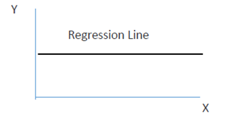
Figure 9. Slope of Regression equation is zero: Regression line is horizontal.
In general, if the slope of the Regression line, or the slope coefficient in the Regression equation, exceeds zero, it suggests that the variable X does explain some of the variation in Y, such that as X increases Y also increases. The Regression line would be upward sloping. Here, one would use a given value of X in the Regression equation to predict the value of Y. The graph sketch in Figure 10 shows that if the slope of the regression line is positive, then, as X increases, Y will also increase.
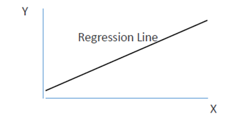
Figure 10. Slope of Regression equation is positive: Regression line slopes upward.
We can view the equation, Ŷ = mx + b, as a sample regression equation corresponding to a population regression equation, Y = Mx + B, which would be based on fitting all the paired values of the population (assuming all possible paired values was sampled). For example, the sample regression equation, CO2 = 115.72492 + 166.90044 GDP, is an estimate of the true population regression equation, Y = Mx + B which would be the regression equation if all countries’ GDP and CO2 emissions standards were to be included.
Here, you will use your sample results to test the hypothesis that the population slope coefficient, M, significantly exceeds zero. If this turns out to be the case, then you can use the sample regression equation to predict values for Y, CO2 emissions, given specific GDP levels (X).
Hypothesis test re Slope of Regression line – Four-step P‑value approach:
| Step 1. | HO: M = 0 (Slope = 0). |
| Step 2. | Use StatCrunch to compute the test statistic and related P‑value. |
Guided Solution 17a
Compute the test statistic and related P‑value (Step 2).
- With the data file Countries.txt open, click the menu sequence Stat → Regression → Simple Linear, to display the Simple Linear Regression window.
- In the X variable box, select GDP.
- In the Y variable box, select CO2.
- In the Perform section:
- Select the Hypotheses tests option.
- Type HO: Slope = 0.
- Select HA: Slope > 0.
Click Compute to display the Simple linear results window, as in Figure 11. Note the T‑Stat and the P‑value corresponding to the slope row in the Parameter estimates table in the Simple linear results window. Test statistic = T‑Stat = 6.2719592 and related P‑value = 0.0001.
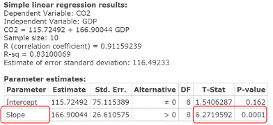
Figure 11. Hypothesis test: Slope of Regression line: test statistic, P‑value.
| Step 3. | As the P‑value = 0.0001 is less than alpha = 0.05, reject HO. |
| Step 4. | The slope of the Regression line significantly exceeds 0. Alternately stated, there is a significant positive linear relation between GDP and CO2 emissions. You can use the Simple linear regression equation to predict CO2 emission levels based on given GDP Levels. |
Guided Solution 17b
Copy the first screen of the Simple linear regression results window with one-sided test statistic and P‑value into your Word file, ComputerLab6A.
- Open your Word file ComputerLab6A.
- Below the bottom item, type the heading: Regression Equation.
- On the next line, copy and paste the Regression output. For help with copying StatCrunch data, see Copying Materials from StatCrunch.
- Save your Word file, ComputerLab6A.
Task 18. Interpretation Question: Hypothesis Test: Slope of Regression Line
In your Word file ComputerLab6A, under the bottom item, Type the four‑steps (P‑value approach) to test the hypothesis related to the slope of the regression line. (If you need help, see the Solution that follows.) Save your Word file, ComputerLab6A.
Solution 18
| Step 1. | HO: M = 0 (Slope = 0). |
| Step 2. | Use StatCrunch to compute the test statistic and related P‑value test statistic T‑Stat = 6.2719592 and related P‑value = 0.0001 |
| Step 3. | As the P‑value = 0.0001 is less than alpha = 0.05, reject HO. |
| Step 4. | The slope of the Regression Line significantly exceeds 0. Alternately stated, there is a significant positive linear relation between GDP and CO2 emissions. You can use the Simple linear regression equation to predict CO2 emission levels based on given GDP Levels. |
Task 19. Construct a 95% prediction interval for CO2 emissions when a country’s GDP level is 3.5 trillion dollars.
In Task 18, we found that the slope of the regression line (coefficient of X in the regression equation) significantly exceeds 0. This finding makes it reasonable to use the regression equation to predict levels of CO2 emissions based on given values of a country’s GDP. Here, you will use StatCrunch to construct a 95% prediction interval for CO2 emissions when a country’s GDP level is 3.5 trillion dollars.
Guided Solution 19a
Compute the 95% prediction interval for CO2 emissions.
- With the data file Countries.txt open, click the menu sequence Stat → Regression → Simple Linear, to display the Simple Linear Regression window.
- In the X variable box, select GDP.
- In the Y variable box, select CO2.
- In Prediction of Y section:
- In the X values box, type 3.5.
- In the Level box, type 0.95.
Click Compute to display the Simple linear results window, as in Figure 12. The 95% prediction interval is displayed in the Predicted values section of the results window: 410.99557 to 988.75734 million metric tons of CO2 emissions.
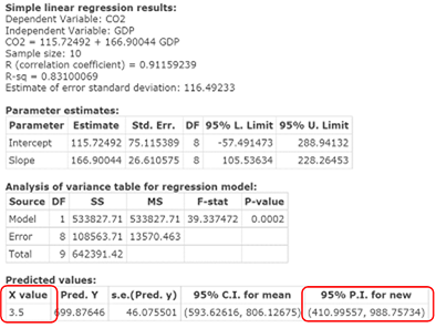
Figure 12. Simple Linear Regression Results window: 95% prediction interval for CO2 emission.
Guided Solution 19b
Copy the first screen of the Simple Linear Results Window into your Word file, ComputerLab6A.
- Open your Word file ComputerLab6A.
- Below the bottom item, type the heading: Prediction Interval.
- On the next line, copy and paste the Simple Linear Results Window output as shown in Figure 12. For help with copying StatCrunch data, see Copying Materials from StatCrunch.
- Save your Word file, ComputerLab6A.
Task 20. Interpretation Questions: 95% Prediction Interval
Copy the question below into your Word file ComputerLab6A, under the bottom item.
Interpret the 95% prediction interval that you just constructed.
Solution:
Based on your review of the Regression output, type your answer in the solution space provided. (If you need help answering the question, see the Solution that follows.) Save your Word file, ComputerLab6A.
Solution 20
- You are 95% confident that, when a country’s GDP is 3.5 trillion dollars, the country’s CO2 emissions will be somewhere between 410.99557 to 988.75734 million metric tons.
Task 21. Exercise 21 from Elementary Statistics, 6th edition
Exercise 21. Age and Blood Pressure

The data are displayed in the StatCrunch data file Ex9_1-21.txt located in the Math 216 group folder at the StatCrunch website. Use StatCrunch to do the following:
- Find the equation of the linear regression line with Ages being the independent variable and Systolic blood pressure being the dependent variable.
- Plot the regression line along with the Scatter plot.
- Compute the Coefficient of Determination, r squared.
- Test to see if the slope of the regression line significantly exceeds zero.
- Construct a 95% prediction interval for Systolic blood pressure for a 50 year old man.
Guided Solution 21a
Here, you will select the options in the Simple Linear Regression window that will answer all parts (a‑e) of this regression analysis.
- Open the StatCrunch data file Ex9_1-21.txt located in the Math 216 group folder at the StatCrunch website.
- Click the menu sequence Stat → Regression → Simple Linear, to display the Simple Linear Regression window.
- In the X variable box, select Age.
- In the Y variable box, select Systolic blood pressure.
- In the Perform section:
- Under Hypothesis tests:
- Type HO: Intercept = 0.
- Select HA: Intercept > 0.
- Under Hypothesis tests:
- In the Graphs section, select Fitted line plot.
- In the Prediction of Y: section:
- In the X values box, type 50.
- In the Level box, type 0.95.
Click Compute to display the Simple Linear Regression Results Window, as in Figure 13.
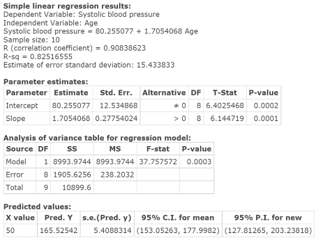
Figure 13. Simple Linear Regression Results window (first screen).
Guided Solution 21b
Copy the first screen of the Simple Linear Results window into your Word file, ComputerLab6A.
- Open your Word file ComputerLab6A.
- Below the bottom item, type the heading: Simple Linear Regression Results, First Screen, Age vs. Systolic Blood Pressure.
- On the next line, copy and paste the Simple Linear Results window output as shown in Figure 13. For help with copying StatCrunch data, see Copying Materials from StatCrunch.
- Save your Word file, ComputerLab6A.
Guided Solution 21c
Plot of regression line fitted to the scatter plot:
Click the right arrow at the bottom of the Simple Linear Results window to display the second screen showing the plot of the Regression Line fitted to the Scatter plot, as in Figure 14.
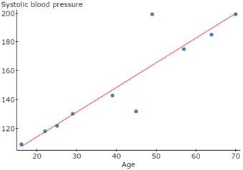
Figure 14. Plot of Fitted Regression Line
Guided Solution 21d
Copy the Plot of Regression Line Fitted to the Scatter plot into your Word file, ComputerLab6A.
- Open your Word file ComputerLab6A.
- Below the bottom item, type the heading: Plot of regression line fitted to the Scatter plot.
- On the next line, copy and paste the graph. For help with copying StatCrunch data, see Copying Materials from StatCrunch.
- Save your Word file, ComputerLab6A.
Task 22. Interpretation Question: Regression Equation and Fitted Line Plot
Copy the questions below into your Word file ComputerLab6A, under the bottom item.
Find the equation of the linear regression line with Ages being the independent variable and Systolic blood pressure being the dependent variable. Interpret the slope coefficient in the equation.
Solution:
Plot the Regression Line along with the Scatter plot. Interpret the upward sloping nature of the Regression Line.
Solution:
Compute the Coefficient of Determination, r squared. Interpret this measure in terms of the relation between Age and Systolic Blood Pressure, as well as in terms of the Fitted Line Plot.
Solution:
Test to see if the slope of the regression line significantly exceeds zero.
Solution:
Construct a 95% prediction interval for Systolic blood pressure for a 50 year old man. Interpret your answer.
Solution:
In the solution spaces provided, type your answers to these questions, based on your review of the StatCrunch Regression output. (If you need help answering the questions, see the Solutions that follow.) Save your Word file, ComputerLab6A.
Solution 22
- Regression equation: Systolic blood pressure = 80.255077 + 1.7054068 Age. The slope coefficient of 1.7054068 suggests that for every one year increase in age, the systolic blood pressure increases by 1.7054068 millimeters of mercury.
- The upward sloping nature of the Regression Line suggests a positive linear relation exists between Age and Systolic blood pressure.
- The Coefficient of Determination = R-sq = 0.82516555. This measure suggests that the variation in Age explains 82.52% of the variation in Systolic Blood Pressure. This also measures the degree to which the Regression Line fits the Scatter plot of (X,Y) values.
Four-step P‑value Test of Hypothesis re. Slope of Regression Line:
Step 1. HO: M = 0 (Slope = 0).
HA: M > 0 (Slope exceeds 0).Step 2. Use StatCrunch to compute the test statistic and related P‑value:
Test statistic = T‑Stat = 6.144719 and related P‑value = 0.0001Step 3. As the P‑value = 0.0001 is less than alpha = 0.05, reject HO.
Step 4. The slope of the Regression Line significantly exceeds 0. Alternately stated, there is a significant positive linear relation between Age and Systolic Blood Pressure. You can proceed to use the Simple Linear Regression Equation to predict Systolic Blood Pressure Levels based on a given Age.
- The 95% prediction interval for Systolic blood pressure for a 50-year-old man is (127.81265,203.23818). You are 95% confident that when a man’s age is 50 years, the man’s systolic blood pressure will be somewhere between 127.81265 to 203.23818 millimeters of mercury.
