Mathematics 216 Computer-oriented Approach to Statistics
Computer Lab 4A
with Guided Solutions (Technology Manual)
Activity 1. Find the Graph, Mean, and Standard Deviation of a population distribution.
Consider the following population experiment:
You write the population values 2, 4, 6, and 8 on four separate slips of paper and place these in a hat. You then randomly select one of those slips of paper. Let the population random variable, X, be the number that you observe on the slip of paper you selected. The probability distribution of X is described in Figure 1 below.
| X | 2 | 4 | 6 | 8 |
| P(X) | .25 | .25 | .25 | .25 |
Figure 1. Population distribution
Task 1. Create the data file PopDistn_5_4.
Open a new StatCrunch data table, and create the file PopDistn_5_4 that displays the values of X in the first column and P(X) in the second column.
Guided Solution 1
Creating the StatCrunch data file PopnDistn_5_4.
- Open StatCrunch.
- In the blank data table, replace the variable names Var1 and Var2 with X and P(X) respectively.
- Under X, enter the four possible values of X shown in Figure 1.
- Under P(X), enter the four different values shown in Figure 1.
Figure 2 shows the probability distribution in StatCrunch.

Figure 2. Population distribution file PopDistn_5_4
- Click the menu sequence Data → Save, and in the Filename box, type PopDistn_5_4
- Click Save to save to your MyData folder.
- Keep data file PopDistn_5_4 open for Task 2.
Task 2. Graph the population distribution and compute the mean and standard deviation of the population distribution.
Use StatCrunch to graph the population distribution and to compute the mean and standard deviation of the population distribution in the data file PopnDistn_5_4.
Guided Solution 2a
- With the file PopnDistn_5_4 open in your data table, click the menu sequence Stat → Calculators → Custom
- In the Values box, select the variable X.
- In the Weights box, select the variable P(X).
Click Compute to display Mean = 5 and Std. Dev. = 2.236068. See Figure 3.
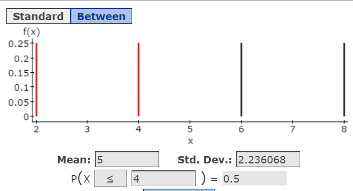
Figure 3. Graph, mean and standard deviation for the population distribution in file PopDistn_5_4
- Note that the graph of the population distribution is also displayed in StatCrunch, showing a uniform distribution, where the probability of all values (height of all bars) is equal at 0.25.
Guided Solution 2b
- Copy the probability distribution graph into a new Word file called ComputerLab4A.
- Type its title, ComputerLab4A.
- Below the title, type: Section 5.4: Population Distribution Example.
- Below that, copy and paste the Graph, Mean and Standard Deviation of Probability Distribution for file PopnDistn_5_4 that you just created in StatCrunch. (For help with copying StatCrunch data, see Copying Materials from StatCrunch.)
- Save the Word file, ComputerLab4A.
Activity 2. Find the Graph, Mean, and Standard Deviation of a sampling distribution.
Consider the following sampling experiment based on the population values described in Activity 1:
With the population values 2, 4, 6, 8 written on separate slips of paper and placed in a hat, you select a sample of two values, with replacement, and observe the sample mean. Let the random variable be Xbar, which consists of the different sample means that you could observe. The probability distribution of Xbar is called the sampling distribution of the sample means and is described in Figure 4 below.
| Xbar | 2 | 3 | 4 | 5 | 6 | 7 | 8 |
| P(Xbar) | 0.0625 | 0.125 | 0.1875 | 0.25 | 0.1875 | 0.125 | 0.0625 |
Figure 4. Sampling distribution of the sample means
Task 3. Create the file SampleDistn_5_4.
Open a new StatCrunch data table and create the file SampleDistn_5_4 that displays the sampling distribution of the sample means, with values of Xbar in the first column and P(Xbar) in the second column.
Guided Solution 3a
- Open StatCrunch.
- In the blank data table, replace the variable names Var1 and Var2 with Xbar and P(Xbar).
- Under Xbar, enter the seven possible values of Xbar shown in Figure 4.
- Under P(Xbar), enter the four different values shown in Figure 4.
Figure 5 describes the probability distribution in StatCrunch.
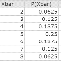
Figure 5. Sampling distribution in file SampleDistn_5_4.
- Click the menu sequence Data → Save, and in the Filename box, type SampleDistn_5_4.
- Click Save to save to your MyData folder.
- Keep this data file open for Task 4.
Guided Solution 3b
Use StatCrunch to graph the sampling distribution and to compute the mean and standard deviation of the sampling distribution in file SampleDistn_5_4.
- With the data file SampleDistn_5_4 open, click the menu sequence Stat → Calculators → Custom.
- In the Values box, select the variable Xbar.
- In the Weights box, select the variable P(X)bar.
Click Compute to display the Mean = 5 and Std. Dev. = 1.5811388. See Figure 6. Note that the graph of the population distribution is also displayed, showing a bell-shaped distribution.
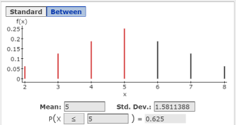
Figure 6. Graph, Mean and Standard Deviation for the sampling distribution in file SampleDistn_5_4
Guided Solution 3c
Copy the sampling distribution into your Word file ComputerLab4A.
- Open the ComputerLab4A Word file.
- Below the bottom item, type the title: Section 5.4: Sampling Distribution Example.
- Below that, copy and paste the Graph, Mean and Standard Deviation of the Sampling Distribution that you just created in StatCrunch for the file SampleDistn_5_4. (For help with copying StatCrunch data, see Copying Materials from StatCrunch.)
- Save your Word file, ComputerLab4A.
Task 4. Interpretation Question: Population distribution vs. sampling distribution
Copy the question below into your ComputerLab4A Word file, under the graph you just pasted.
Based on your review of the population and sampling distribution examples, type your answers in the solutions spaces provided. (If you need help answering these questions, see the Solutions section that follows them.)
Compare the graph of the population distribution for the file PopDistn_5_4 with the graph of the sampling distribution for the file SampleDistn_5_4. Are your results consistent with the Central Limit Theorem? Explain.
Solution:
In comparing the mean and standard deviation of the population distribution for the file PopDistn_5_4 with the mean and standard deviation of the sampling distribution for the file SampleDistn_5_4, are your results consistent with the Central Limit Theorem? Explain.
Solution:
Remember to save your Word file, ComputerLab4A.
Solution 4
- Yes, because the sampling distribution is bell-shaped even though the population is uniform.
- Yes, because the mean of the sampling distribution = mean of the population mean = 5. As well, the standard deviation of the sampling distribution = (Population Standard Deviation/ Square Root of Sample Size) = (2.236068/Sqrt2) = (2.236068/ 1.4142) = 1.58114.
Activity 3. Approximate the Graph, Mean, and Standard Deviation of a Sampling Distribution of Sample Means through Simulation
Task 5. Generate 10,000 repetitions of a sampling experiment.
Use StatCrunch to open the file PopDistn_5_4 and generate 10,000 repetitions of the following sampling experiment. Drawing on the population values 2, 4, 6, 8, you will randomly select a sample of two values, with replacement, and observe the sample mean. StatCrunch will simulate this experiment 10,000 times, so that 10,000 sample means will be created in one column of the data table.
Guided Solution 5
Simulate 10,000 repetitions of the sampling experiment.
- Open the StatCrunch data file Pop_Distn_5_4. (For help, see Accessing and Working in StatCrunch on the course home page.)
- Click the menu sequence Data → Sample.
- In the Sample Columns window that displays:
- In Select columns, select X.
- In the Sample size box, type 2.
- In the Number of samples box, type 10000.
- in the Sampling Options section, select:
- Sample with replacement
- Sample all columns at one time
- In the Store samples section:
- Select: Compute statistic for each sample.
In the Build box, type: mean(“Sample(X)”). See Figure 7.
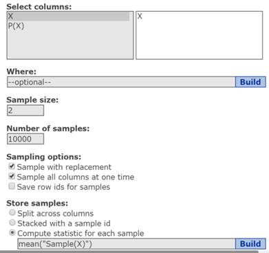
Figure 7. Sample columns window for simulating 10,000 sample means.
- Click Compute. This will add a new column called Mean(Sample(X)), which shows 10,000 sample means (in 10,000 rows). Note that different sets of sample means will be generated for different individuals.
- Click save to save the changes you have made to this file.
Task 6. Compute mean and standard deviation
Use StatCrunch to compute the mean and standard deviation of the 10,000 sample means you just generated. Compute the mean of the new variable “mean(Sample(X))”.
Guided Solution 6
- Open the StatCrunch data file Pop_Distn_5_4. (For help, see Accessing and Working in StatCrunch on the course home page.)
- With the column mean(Sample(X)) displayed in StatCrunch, click the menu sequence Stat → Summary Stats → Columns.
- In the Summary Stats window that displays:
- In the Select columns box, select the variable mean(Sample(x)).
- In the Statistics box, select mean and std. dev. (using the Ctrl key).
- Click Compute to display mean (approximately 5.0) and std. dev. (approximately 1.5). Note that, because different sets of sample means were generated for different individuals, the mean and standard deviation will also differ.
Task 7. Interpretation Question: Compare Activity 2 results to Activity 3 results.
Copy the question below into your ComputerLab4A Word file, under the bottom item.
Compare the StatCrunch results observed in Activity 2 and Activity 3.
Solution:
Based on your review of the results in Activity 2 and Activity 3, type your answer in the solution space provided. (If you need help answering the question, see the Solution that follows.) Remember to save your Word file, ComputerLab4A.
Solution 7
- The mean and standard deviation of the 10,000 means generated in Activity 3 is approximately equal to the mean and standard deviation of the sampling distribution in Activity 2, as one would expect. Recall that the mean and standard deviation of a distribution can be approximated by “long run averages”.
Task 8. Create a relative frequency histogram.
Use StatCrunch to create a relative frequency histogram for the 10,000 sample means you generated. Create a relative frequency for the variable “mean(Sample(X))”.
Guided Solution 8
- With the data file PopDistn_5_4 open and the column mean(Sample(X)) displayed, click the menu sequence Graph → Histogram.
- In the Select columns box, select the variable mean(Sample(x)).
- In the Type box, select Relative Frequency.
Click Compute to display a relative frequency graph similar to Figure 8. Note that different individuals will get a slightly different histogram.
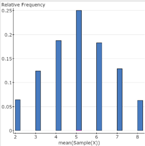
Figure 8. Relative frequency histogram of the 10,000 sample means
Task 9. Interpretation Question: Assess the relative frequency histogram results based on the central limit theorem.
Copy the question below into your ComputerLab4A Word file, under the bottom item.
Is the relative frequency histogram created for the 10,000 sample means consistent with the central limit theorem?
Solution:
Based on your review of the results observed in Activity 3, type your answer in the solution space provided. (If you need help answering the question, see the Solution that follows.) Remember to save your Word file, ComputerLab4A.
Solution 9
- Yes, the relative frequency histogram created for the 10,000 sample means is approximately bell-shaped, despite the fact that the population distribution is NOT bell-shaped.
Activity 4. Compute confidence intervals for the population mean: Population standard deviation known.
Chapter 6 of your eText notes that, for cases in which the population standard deviation is known and either the population is normal or the sample size is greater than 30, you can use the standard normal variable, z, in computing the confidence interval. The following questions are examples of such cases.
Task 10. Example 1 from Elementary Statistics, 6th edition
Example 1 Number of Hours Worked
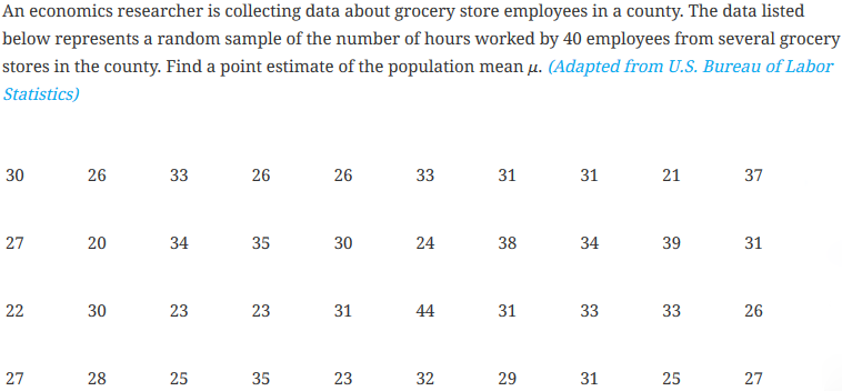
The data has been stored in StatCrunch in a data file Grocery.txt stored in the AU Math216 2020 groups folder at the Statcrunch.com website. Based on this sample data, use StatCrunch to construct these three Confidence Intervals for the mean number of hours worked by all grocery store workers in this city:
- a 99% Confidence Interval
- a 90% Confidence Interval
- a 75% Confidence Interval
Guided Solution 10a
Construct a 99% Confidence Interval for mean number of hours worked.
- Open the data file Grocery.txt for Example 1 stored in the AU Math216 2020 groups folder at the Statcrunch.com website. (For help, see Accessing and Working in StatCrunch on the course home page.)
- With the data table Grocery.txt open, click the menu sequence Stat → Z Stats → One Sample → With Data. (“With Data” means that you are working with the original sample data.)
- In the One Sample Z window that displays:
- In the Select columns box, click Number of hours.
- In the Standard deviation box, type 7.9.
- In the Perform section, select Confidence interval for μ.
In the Level box, type 0.99. See Figure 9.
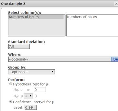
Figure 9. One Sample Z window.
Click Compute to display the confidence interval as shown in Figure 10.

Figure 10. 99% confidence interval for mean hours worked
Guided Solution 10b
Copy the Sampling Distribution into your Word file ComputerLab4A.
- Open the ComputerLab4A Word file.
- Below the bottom item, type the title: Section 6.1: Confidence Interval for Population Mean: Populations Standard Deviation Known.
- On the next line, type the subtitle: 99% Confidence Interval.
- Below that, copy and paste the confidence interval table you just created (as in Figure 10). (For help with copying StatCrunch data, see Copying Materials from StatCrunch.)
- Save your Word file, ComputerLab4A.
Guided Solution 10c
Construct a 90% confidence interval for mean number of hours worked.
- Open the data file Grocery.txt for Example 1 in Section 6.1. (For help, see Accessing and Working in StatCrunch on the course home page.)
- With the data table Grocery.txt open, click the menu sequence Stat → Z Stats → One Sample → With Data.
- In the One Sample Z window that displays:
- In the Select columns box, click Number of hours.
- In the Standard deviation box, type 7.9.
- In the Perform section, select Confidence interval for μ.
- In the Level box, type 0.90.
Click Compute to display the confidence interval as in Figure 11.

Figure 11. 90% confidence interval for mean hours worked.
Guided Solution 10d
Copy the Sampling Distribution into your Word file ComputerLab4A.
- Open the ComputerLab4A Word file.
- Below the bottom item, type the subtitle: 90% Confidence Interval.
- Below that, copy and paste Confidence Interval Table you just created (as in Figure 11). (For help with copying StatCrunch data, see Copying Materials from StatCrunch.)
- Save your Word file, ComputerLab4A.
Guided Solution 10e
Construct a 75% Confidence Interval for Mean Number of Hours Worked.
- With the data table Grocery.txt open, click the menu sequence Stat → Z Stats → One Sample → With Data.
- In the One Sample Z window that displays:
- In the Select columns box, click Number of hours.
- In the Standard deviation box, type 7.9.
- In the Perform section, select Confidence interval for μ.
- In the Level box, type 0.75.
Click Compute to display the confidence interval as in Figure 12.

Figure 12. 75% confidence interval for mean hours worked.
Guided Solution 10f
Copy the Confidence Interval into your Word file, ComputerLab4A.
- Same steps as in Guide Solution 10d.
Task 11. Interpretation Questions: Confidence intervals
Copy the questions below into your ComputerLab4A Word file, under the bottom item.
Interpret, in words, the meaning of the 99% confidence interval you just computed for 6.1
Solution:
Interpret, in words, the meaning of the 90% confidence interval you just computed for 6.1
Solution:
Based on your review of the confidence interval tables, type your answers in the solution spaces provided. (If you need help answering these questions, see the Solution section that follows.) Remember to save your Word file, ComputerLab4A.
Solution 11
- With 99% confidence, you can say that the population mean number of hours worked is between 26.38 and 32.82 hours.
- With 90% confidence, you can say that the population mean number of hours worked is between 27.55 and 31.65 hours.
Task 12. Interpretation Question: Confidence Interval Width and Level of Confidence
Copy the question below into your ComputerLab4A Word file, under the bottom item.
How does the width of the confidence interval (called the precision of the interval estimate) change as the level of confidence decreases?
Solution:
Based on your review of the confidence interval table, type your answer in the solution space provided. (If you need help answering the question, see the Solution that follows.) Remember to save your Word file, ComputerLab4A.
Solution 12
- The width of the confidence interval decreases as the level of confidence decreases.
Task 13. Exercise 37 from Elementary Statistics, 6th edition
Exercise 37. Replacement Costs

Guided Solution 13a
Construct a 95% confidence interval for mean repair costs.
- Open a new data table in StatCrunch.
- Click the menu sequence Stat → Z Stats → One Sample → With Summary.
- In the One Sample Z Summary window that displays:
- In the Sample mean box, type 2650.
- In the Standard deviation box, type 425.
- In the Sample size box, type 50. In the Perform section, select Confidence Interval for μ.
- In the Level box, type 0.95. See Figure 13.
Click Compute to display the confidence interval as in Figure 13.

Figure 13. 95% Confidence interval for repair costs.
Guided Solution 13b
- Open the ComputerLab4A Word file.
- Below the bottom item, type the title: 95% Confidence Interval Estimate for Mean Car Transmission Repairs.
Copy the Confidence Interval into your Word file, ComputerLab4A.
Same steps as in the previous example:
Task 14. Interpretation Question: Exercise 37
Copy the question below into your ComputerLab4A Word file, below the bottom item:
Suppose the auto repair company under study claims that its average auto transmission repair costs are typically below $2500. Does the confidence interval that you computed support this claim?
Solution:
Based on your review of the confidence interval table, type your answer in the solution space provided. (If you need help answering the question, see the Solution that follows.) Remember to save your Word file, ComputerLab4A.
Solution 14
- No. The confidence interval that you constructed can be interpreted as follows: With 95% confidence, you can say that the average auto transmission repair costs are somewhere between $2532.19 and $2767.80. As the company’s claim is outside the confidence interval, there is only a 5% probability that the claim is valid.
Activity 5. Computing Confidence Intervals for the Population Mean: Population Standard Deviation Unknown
Chapter 6 notes that, in cases where the population standard deviation is unknown and either the population is normal or the sample size is greater than 30, you can use the variable, t, in computing the confidence interval. The following questions are examples of such cases.
Task 15. Exercise 29 from Elementary Statistics, 6th edition
Exercise 29. Annual Earnings
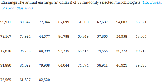
Data on the annual earnings of a sample of 35 randomly selected microbiologists has been stored in StatCrunch in a data file Ex6_2-29.txt stored in the AU Math216 2020 groups folder at the Statcrunch.com website.
Guided Solution 15a
Construct a 98% Confidence Interval for mean annual earnings of microbiologists.
- Open the data file Ex6_2-29.txt Exercise 29 in Section 6.2 stored in the AU Math216 2020 groups folder at the Statcrunch.com website. (For help, see Accessing and Working in StatCrunch on the course home page.)
- Click the menu sequence Stat → T Stats → One Sample → With Data.
- In the One Sample T window that displays:
- In the Select columns box, select Annual earnings (in dollars).
- In the Perform section, select Confidence Interval.
- In the Level box, type 0.98.
Click Compute to display the confidence interval as in Figure 14.

Figure 14. 98% Confidence Interval for Annual Earnings of Microbiologists
Guided Solution 15b
Here, you will open the ComputerLab4A Word file and then, below the subtitle, copy and paste the Confidence Interval Table that you just created in StatCrunch (as in Figure 14). You will then save this document under the file name ComputerLab4A.
Copy the Confidence Interval into your Word file, ComputerLab4A.
- Below the bottom item, type the title: Section 6.2: Confidence Interval for Population Mean: Populations Standard Deviation Unknown.
- On the next line, type the subtitle 98% Confidence Interval.
- Same steps as in the previous example: Options → Copy → Ctrl+A → Ctrl+C → Ctrl+V → etc.
Task 16. Interpretation Question: Exercise 29 in Section 6.2
Copy the question below into your ComputerLab4A Word file, under the bottom item.
Interpret, in words, the meaning of the confidence interval just computed for 6.2 Exercise 29.
Solution:
Based on your review of the confidence interval table, type your answer in the solution space provided. (If you need help answering the question, see the Solution that follows.) Remember to save your Word file, ComputerLab4A.
Solution 16
- With 98% confidence, you can say that the population mean annual earnings of microbiologists is between $65,602.69 and 78,333.42.
Task 17. Exercise 17 from Elementary Statistics, 6th edition
Exercise 17. Commute Time

Assuming the population is normally distributed, construct a 95% confidence interval for the population mean commute time.
Guided Solution 17a
Construct a 95% Confidence Interval for mean commute time.
- Open a new data file in StatCrunch.
- Click the menu sequence Stat → T Stats → One Sample → With Summary. (“With Summary” means that you are working with summarized data such as the mean and standard deviation.)
- In the One Sample T window that displays:
- In the Sample mean box, type 35.5.
- In the Sample std. dev. box, type 7.2.
- In the Sample Size box, type 8.
- In the Perform section, select Confidence interval for μ.
In the Level box, type 0.95. See Figure 15.
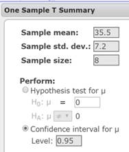
Figure 15. 95% One Sample T summary window.
Click Compute to display the confidence interval as in Figure 16.

Figure 16. 95% Confidence Interval for commute time.
Guided Solution 17b
Exercise 17 in Section 6.2: Construct a 99% Confidence Interval for Mean Commute Time
- Open a new data table in StatCrunch.
- Click the menu sequence Stat → T Stats → One Sample → With Summary (“With Summary” means that you are working with summarized data such as the mean and standard deviation).
- In the One Sample T Summary window that displays:
In the Sample Mean box, type 35.5
In the Standard Deviation box, type 7.2
In the Sample Size box, type 8
In the Perform section, select Confidence Interval
In the Level box, type .99 Click Compute to display the confidence interval as in Figure 17.

Figure 17. 99% Confidence Interval for Mean Commute Time
Guided Solution 17c
- Copy the 95% and 99% Confidence Intervals into your Word file, ComputerLab4A.
- Below the bottom item, type the title: Section 6.2: Confidence Interval for Population Mean: Populations Standard Deviation Unknown.
- On the next line, type the subtitle: 95% and 99% Confidence Interval
- Below that, copy and paste the Confidence Interval Tables. you just created.
- Save this document under the file name ComputerLab4A.
Task 18. Interpretation Question: Exercise 17 in Section 6.2
Copy the question below into your ComputerLab4A Word file, under the bottom item.
Interpret, in words, the meaning of the confidence interval just computed for 6.2 Exercise 17.
Solution:
Based on your review of the confidence interval table, type your answer in the solution space provided. (If you need help answering the question, see the Solution that follows.) Remember to save your Word file, ComputerLab4A.
Solution 18
- With 95% confidence, you can say that the mean population commute time is between 29.48 and 41.52 minutes. With 99% confidence, you can say that the mean population commute time is between 26.59 and 44.41 minutes. Note that the larger the level of confidence, the wider the confidence interval.
Activity 6. Find the Minimum Sample Size to Estimate a Population Mean
Chapter 6 of your text notes that, given a confidence level, the population standard deviation, and a maximum tolerable margin of error, E, the z value is used in the formula to find the minimum sample size to estimate a population mean. If the population standard deviation is unknown, one can use the sample standard deviation if the sample size is at least 30.
In using StatCrunch to find the minimum sample size, instead of specifying the maximum tolerable error, E, we will us the maximum tolerable confidence interval, which is 2 × E.
Task 19. Example 6 from Elementary Statistics, 6th edition
Review Example 6. Assume that the population standard deviation is 7.9 hours.
Example 6 Hours Worked
An economics researcher wants to estimate the mean number of hours worked by all grocery store employees in the county. How many employees must be included in the sample to be 95% confident that the sample mean is within 1.5 hours of the population mean?
Guided Solution 19a
Find the minimum sample size to estimate the population mean hours worked.
- Open a new data table in StatCrunch.
- Click the menu sequence Stat → Z Stats → One Sample → Power/Sample Size.
- In the window that displays, click the Confidence Interval Width button.
- In the Required parameters section:
- In the Confidence level box, type 0.95.
- In the Standard deviation box, type 7.9
In the Enter One section, in the Width box, type 3 (which is the tolerable error E of 1.5, multiplied by 2). See Figure 18.

Figure 18. Confidence interval width window
Click Compute to display that the Sample size is 107. See Figure 19.

Figure 19. Confidence interval width window with sample size found.
Guided Solution 19b
Copy the Confidence Interval Width window into your Word file, ComputerLab4A.
- Open the ComputerLab4A Word file,
- Below the bottom, type the heading: Finding the Minimum Sample Size to Estimate the Population Mean Hours Worked.
- On the next line, copy and paste the Confidence Interval Width window. (For help with copying StatCrunch data, see Copying Materials from StatCrunch.)
- Save your file, ComputerLab4A.
Task 20. Interpretation Question: Example 6 in Section 6.1
Copy the question below into your ComputerLab4A Word file, under the bottom item.
Interpret, in words, the meaning of the sample size value just computed for 6.1 Example 6.
Solution:
Based on your review of the confidence interval width window, type your answer in the solution space provided. (If you need help answering the question, see the Solution that follows.) Remember to save your Word file, ComputerLab4A.
Solution 20
- To be 95% confident that the sample mean will be within 1.5 hours of the population mean hours worked, 107 employees need to be randomly sampled.
Task 21. Exercise 47 from Elementary Statistics, 6th edition
Exercise 47. Minimum Sample Size

Guided Solution 21
Find the minimum sample size to estimate the population mean.
- Follow Guided Solution 19a, but use a standard deviation 4.8 and a width of 2 × 1 = 2. The sample size that you find should be 89.
Activity 7. Compute a confidence interval for the population proportion.
Here, you will use StatCrunch to compute confidence interval estimates for population proportions.
Task 22. Example 1 from Elementary Statistics, 6th edition
Example 1 Smartphone Ownership
In a survey of 1000 teens, 372 stated that they own smartphones. Construct a 95% confidence interval estimate for the population proportion of teens who own smartphones.
Guided Solution 22a
- Open a new data table in StatCrunch.
- Click the menu sequence Stat → Proportion Stats → One Sample → With Summary.
- In the One Sample Prop Summary window that displays:
- In the # of successes box, type 372.
- In the # of observations box, type 1000.
- In the Perform section, select Confidence Intervals for p
In the Level box, type 0.95. See Figure 20.
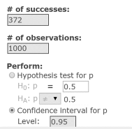
Figure 20. One Sample Prop Summary Window
Click Compute to display the confidence interval of 0.3420 to 0.40195. See Figure 21.

Figure 21. Confidence interval estimate for the population proportion that owns smartphones.
Guided Solution 22b
Copy the Confidence Interval Table into your Word file, ComputerLab4A
- Open the ComputerLab4A Word file.
- Below the bottom, type the heading: Computing the Confidence Interval Estimate for the Population Proportion Who Own Smartphones.
- On the next line, copy and paste the Confidence Interval Width table. (For help with copying StatCrunch data, see Copying Materials from StatCrunch.)
Save your file, ComputerLab4A.
Task 23. Interpretation Question: Example 2 in Section 6.3
Copy the questions below into your ComputerLab4A Word file, under the bottom item.
Interpret the confidence interval just constructed, in percentage terms.
Solution:
Does the confidence interval constructed support a recent claim that the majority of teens own smartphones?
Solution:
Based on your review of the confidence interval width table, type your answers in the solution spaces provided. (If you need help answering the question, see the Solution that follows.) Remember to save your Word file, ComputerLab4A.
Solution 23
- You can state with 95% confidence that between 34.2043% and 40.1957% of all teens own smartphones.
- No. The upper limit of the 95% confidence interval is 40.1957%, which falls short of being over 50% (i.e., falls short of a majority).
Task 24. Exercise 13 from Elementary Statistics, 6th edition
Exercise 13. Going Green

Construct a 99% confidence interval for the population proportion of adults who have started to pay bills online.
Guided Solution 24
- Follow the guided solution steps in Task 22, but use # successes of 1435, # observations of 3110, and confidence level of 0.99. The interval computed should be: 0.4383 to 0.4844.
Activity 8. Find the minimum sample size to estimate a population proportion.
Chapter 6 of your text notes that, given a confidence level, the sample proportion , and a maximum tolerable margin of error, E, the z value is used in the formula used to find the minimum sample size to estimate a population proportion.
In using StatCrunch to find the minimum sample size, instead of specifying the maximum tolerable error, E, we will use the maximum tolerable confidence interval, which is 2 × E.
Task 25. Example 4 from Elementary Statistics, 6th edition
Example 4 Population Proportion Who Vote

Find the minimum number of voters that you need to sample
- assuming that you have no preliminary estimate of the desired proportion.
- assuming that the preliminary estimate of the proportion is a sample proportion of 0.31.
Guided Solution 25a
Find the minimum sample size to estimate the population proportion of voters who will vote your candidate. You have no preliminary estimate of the desired proportion.
- Open a new data table in StatCrunch.
- Click the menu sequence Stat → Proportion Stats → One Sample → Power/Sample Size.
- In the window that displays, click the Confidence Interval Width button.
- In the Required parameters section:
- In the Confidence level box, type 0.95.
- In the Target proportion box, type 0.5.
In the Enter one section: in the Width box, type 0.06 (which is the tolerable error E of 0.03 multiplied by 2). See Figure 22.

Figure 22. Confidence interval width window.
Click Compute to display Sample size of 1068,as in Figure 23.

Figure 23. Confidence interval width window with sample size found.
Guided Solution 25b
Copy the Confidence Interval Width window into your Word file, ComputerLab4A. For help with copying StatCrunch data, see Copying Materials from StatCrunch.
- Use the heading: Finding the Minimum Sample Size to Estimate the Population Proportion of Voters Who Will Vote Your Candidate-No Preliminary Estimate.
- On the next line, copy and paste the Confidence Interval Width Windowcreated in StatCrunch into this document.
- Save your Word file, ComputerLab4A.
Guided Solution 25c
Find the minimum sample size to estimate the population proportion of voters who will vote your candidate. You have a preliminary estimate of 0.31.
- Follow the steps in Guided Solution 25a, but use the target proportion 0.31.
- The solution should be a sample size of 913 voters must be sampled.
Task 26. Interpretation Question: 6.3 Example 4
Copy the question below into your ComputerLab4A Word file, under the bottom item.
In which situation will one get a lower sample size requirement: when no preliminary estimate is used, or when you have a reasonable preliminary estimate to use?
Solution:
Based on your review of the confidence interval width windows, type your answer in the solution space provided. (If you need help answering the question, see the Solution that follows.) Remember to save your Word file, ComputerLab4A.
Solution 26
- A smaller sample size will be required if you have a reasonable preliminary estimate of the population proportion.
