Mathematics 216 Computer-oriented Approach to Statistics
Computer Lab 4B
with Guided Solutions (Technology Manual)
With the aid of the Guided Solutions, use StatCrunch to work through each of the following Activities in your text that relate to Chapter 7 Hypothesis Testing with One Sample.
Activity 1. Use a four-step P‑value approach for hypothesis tests.
In testing hypothesis in the computer component of this course, we will use the following four-step P‑value approach:
| Step 1. | Specify HO and HA. |
| Step 2. | Use StatCrunch to compute the appropriate test statistic and related P‑value. |
| Step 3. | Make a decision based on comparing the P‑value with the level of significance, alpha, as follows: |
| Step 4. | Interpret the decision in Step 3 in the context of the original claim. |
The four-step P‑value approach is applied in answering Exercise 27 in Section 7.3.
Task 1. Exercise 27 from Elementary Statistics, 6th edition
Exercise 27. Class Size

Test the university’s claim, that the mean class size of full-time faculty is fewer than 32 students, at a level of significance of 5%. The data collected has been stored in a data file called Ex7_3-27.txt, in the StatCrunch Math 216 group.
| Step 1. | Specify the hypotheses: |
| Step 2. | Use StatCrunch to compute the appropriate test statistic and related P‑value. |
Guided Solution 1
Use StatCrunch to compute the test statistic and related P‑value that will be used to test the hypothesis (this is Step 2). As the population standard deviation is unknown, you will use the t statistic (not the z statistic) in this test.
- Open the data file Ex7_3-27.txt. (For help, see Accessing and Working in StatCrunch on the course home page.)
- Click the menu sequence Stat → T Stats → One Sample → With Data,
- In the Select columns box, select the variable class size.
- In the Perform section, select Hypothesis test for μ (mean).
- In the HO μ = box, type 32.
In the HA μ box, select < to specify the hypothesis as Mean < 32. See Figure 1.
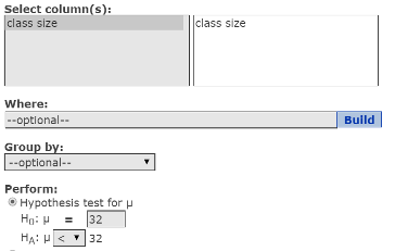
Figure 1. One sample t window
Click Compute to display theHypothesis test results window, as shown in Figure 2. As the hypothesis test results window indicates, the test statistic = t = −1.9427588; related P‑value = 0.0344.

Figure 2. Hypothesis test results window.
| Step 3. | As the P‑value = 0.0344 is less than alpha = 0.05, reject HO. |
| Step 4. | Mean class size is less than 32 students per class. |
Activity 2. Test the assumption that the population is normally distributed.
When using the T-stat in conducting the test of hypothesis in Task 1, you assumed that the population is normally distributed (as the sample size is only 18 class sizes, which is fewer than 30).
In the computer component of this course, you will be responsible for conducting the following Shapiro-Wilk Test of Hypothesis to determine if the population appears to be normally distributed.
Shapiro-Wilk Test for Normality:
| Step 1. | Specify the hypotheses: |
| Step 2. | Use StatCrunch to compute the Shapiro-Wilk test statistic and related P‑value. |
| Step 3. | Make a decision based on comparing the P‑value with the level of significance, alpha, as follows: |
| Step 4. | State your conclusion. |
Task 2. Use the Shapiro-Wilk Test for Normality to determine if the sample of 18 class sizes appears to come from a normal population.
Use the Shapiro-Wilk Test for Normality to determine if the sample of 18 class sizes in Exercise 27 Section 7.3 appears to come from a normal population. Assume a 5% level of significance for this test.
| Step 1. | Specify the hypotheses: |
| Step 2. | Use StatCrunch to compute the Shapiro-Wilk test statistic and related P‑value. (Continued below.) |
Guided Solution 2
Use StatCrunch to Compute the Shapiro-Wilk test statistic and P‑value (Step 2).
- With the data file Ex7_3-27.txt open, click the menu sequence Stat → Goodness-of-fit → Normality Test.
- In the Select columns box, select the variable class size.
In the Test box, select Shapiro-Wilk. See Figure 3.
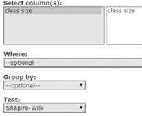
Figure 3. Normality test window.
Click Computeto display theHypothesis test results window, as shown in Figure 4. The test statistic = 0.92879777; P‑value = 0.185.

Figure 4. Shapiro-Wilk results window.
| Step 3. | As the P‑value = 0.185 exceeds alpha = 0.05, do not reject HO. |
| Step 4. | You cannot conclude that the population is not normally distributed (therefore, the assumption of normal population is reasonable). As a result, you can feel confident in your conclusion in the previous hypothesis test regarding class size, that the mean class size is less than 32 students per class. |
Activity 3. Hypothesis testing for the mean with population standard deviation unknown.
Task 3. Exercise 21 from Elementary Statistics, 6th edition
Exercise 21. Annual Salary

Test the employment information service’s claim, at a level of significance of 5%. The data is stored in the StatCrunch data file Ex7_3-21.txt, which is available in the Math 216 group data file.
| Step 1. | Specify the hypotheses: |
| Step 2. | Use StatCrunch to compute the appropriate test statistic and related P‑value. |
Guided Solution 3a
Use StatCrunch to compute the test statistic and related P‑value that will be used to test the hypothesis. As the population standard deviation is unknown, you will use the t statistic (not the z statistic) in this test.
- Open the StatCrunch data file Ex7_3-21.txt. (For help, see Accessing and Working in StatCrunch on the course home page.)
- Click the menu sequence Stat → T Stats → One Sample → With Data.
- In the Select columns box, select the variable salary.
- In the Perform section of the window select Hypothesis test for μ.
- In the HO: μ box, type 26000.
In the HA: μ box, select ≠ to specify the alternate hypothesis as: Mean ≠ 26000. See Figure 5.
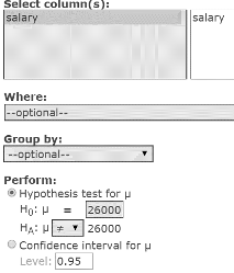
Figure 5. One sample T window.
Click Compute to display the Hypothesis test results, as shown in Figure 6.

Figure 6. Hypothesis test results window.
| Step 2. | (continued): As the Hypothesis test results window indicates, the test statistic = t = −0.64074779; related P‑value = 0.5377. |
| Step 3. | As the P‑value = 0.5377 exceeds alpha = 0.05, do not reject HO. |
| Step 4. | You cannot reject the claim that mean salaries equal $26,000. |
Guided Solution 3b
Copy the Hypothesis test results table into your Word file, ComputerLab4B.
- Create a new Word file called ComputerLab4B.
- Type the title: Hypothesis Tests for a Population Mean- Population Standard Deviation Unknown.
- On the next line, copy and paste the Hypothesis test results table you created. For help with copying StatCrunch data, see Copying Materials from StatCrunch.
- Save your Word file, ComputerLab4B.
Task 4. Interpretation Question: Hypothesis test for the population mean—population standard deviation unknown
Copy the four-step P‑value approach for hypothesis tests and the question below into your ComputerLab4B Word file, below the bottom item. (If you need help answering the question, see the Solution that follows.)
Is it necessary to conduct a normality test on the sample data?
Solution:
Remember to save your Word file, ComputerLab4B.
Solution 4
| Step 1. | HO: Population mean equals 26,000. |
| Step 2. | Test statistic = t = −0.64074779; related P‑value = 0.5377. |
| Step 3. | As the P‑value of 0.5377 exceeds alpha = 0.05, do not reject HO. |
| Step 4. | We cannot reject the claim that average salaries equal 26,000. |
It is necessary to conduct a normality test, as the sample size is less than 30.
Note that, as the sample size is less than 30, we assumed that the sample came from a normally distributed population in order to use the t-statistic in our test of hypothesis regarding mean salaries. In the next exercise, we will test this assumption.
Task 5. Use the Shapiro-Wilk test for normality.
Use the Shapiro-Wilk Test for Normality to determine if the sample of 10 salaries in Exercise 21 Section 7.3 appears to come from a normal population. Assume a 5% level of significance for this test.
| Step 1. | Specify the hypotheses: |
| Step 2. | Use StatCrunch to compute the Shapiro-Wilk test statistic and related P‑value. |
Guided Solution 5a
- With the data file Ex7_3-21.txt open, click the menu sequence Stat → Goodness-of-fit → Normality Test.
- In the Select columns box, select the variable Salary.
- In the Test box, select Shapiro-Wilk.
Click Compute to display theShapiro-Wilk results table, as shown in Figure 7. The test statistic = 0.97214064; P‑value = 0.91.

Figure 7. Shapiro-Wilk results table.
| Step 3. | As the P‑value = 0.91 exceeds alpha = 0.05, do not reject HO. |
| Step 4. | You cannot conclude that the population is not normally distributed (therefore, the assumption of normal population is reasonable). As a result, you can feel confident in your conclusion in the previous hypothesis test regarding salaries of males without high school education. |
Guided Solution 5b
Copy the Shapiro-Wilk results table into your Word file, ComputerLab4B.
- Type the title: Shapiro-Wilk Normality Test.
- On the next line, copy and paste the Hypothesis test results table you created. For help with copying StatCrunch data, see Copying Materials from StatCrunch.
Save your Word file, ComputerLab4B.
Task 6. Interpretation Question: Shapiro-Wilk Normality Test
Copy the four-step P‑value approach for normality tests below into your ComputerLab4B Word file, below the bottom item. (If you need help answering the question, see the Solution that follows.)
Remember to save your Word file, ComputerLab4B.
Solution 6
| Step 1. | HO: The population is normally distributed. |
| Step 2. | Test statistic = t =.97214064; related P‑value = 0.91 |
| Step 3. | As the P‑value of 0.91 exceeds alpha = 0.05, do not reject HO. |
| Step 4. | You cannot conclude that the population is not normally distributed (therefore, the assumption of normal population is reasonable). As a result, you can feel confident in your conclusion in the previous hypothesis test regarding salaries of males without high school education. |
Task 7. Exercise 17 from Elementary Statistics, 6th edition
Exercise 17. Credit Card Balances

At a level of significance of 5%, can you support the company’s claim?
| Step 1. | Specify the hypotheses: |
| Step 2. | Use StatCrunch to compute the appropriate test statistic and related P‑value. |
Guided Solution 7a
Use StatCrunch to compute the test statistic and related P‑value (this is Step 2) that will be used to test the hypothesis for Exercise 17 in Section 7.3. As the population standard deviation is unknown, you will use the t statistic (not the z statistic) in this test.
- With a new data table open in StatCrunch, click the menu sequence Stat → T Stats → One Sample → With Summary.
- In the One Sample T Summary window that displays:
- In the Sample mean box, type 5122.
- In the Sample std. dev. box, type 625.
- In the Sample size. box, type 37.
- In the Perform section:
- Select the Hypothesis test option.
- In the HO: μ = box, type 5000.
In the HA box, select >. See Figure 8.
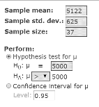
Figure 8. One Sample T Summary window.
Click Compute to display the Hypothesis test results window, as in Figure 9. As the Hypothesis test results window indicates, the test statistic = t = 1.1873552; related P‑value = 0.1214.

Figure 9. Hypothesis tests results window.
| Step 3. | As the P‑value = 0.1214 exceeds alpha = 0.05, do not reject HO. |
| Step 4. | The sample does not support the claim that the mean credit card debt exceeds $5000. |
Guided Solution 7b
Copy the Hypothesis test results table into your Word file, ComputerLab4B.
- Type the title: Hypothesis Tests for Population Mean-Pop SD Unknown-Summary Data
- On the next line, copy and paste the Hypothesis test results table you created. For help with copying StatCrunch data, see Copying Materials from StatCrunch.
- Save your Word file, ComputerLab4B.
Task 8. Interpretation Question: Hypothesis Test for the Population Mean—Population Standard Deviation Unknown
Type the four-steps (P‑value approach) to test the hypothesis related to Hypothesis Test Results Table below the bottom item in your Word file CompterLab4B. (If you need help, see the Solution section that follows.)
Do we need to conduct the normality test for the credit card hypothesis test?
Remember to save your Word file, ComputerLab4B.
Solution 8
| Step 1. | HO: μ less than or equal to $5,000. |
| Step 2. | Test statistic = t = 1.1873552; related P‑value = 0.121 |
| Step 3. | As the P‑value of 0.1214 exceeds alpha = 0.05, do not reject HO. |
| Step 4. | We cannot support the claim that the average credit card debt exceeds $5,000. |
Note that, as the sample size is greater than 30, we do not need to conduct a normality test.
Activity 4. Hypothesis Tests Involving a Single Population Proportion
Here, you will use the four-step P‑value approach in testing hypotheses regarding a single population proportion.
You will open up a StatCrunch data file Field Goal Data for the 2013 NFL Season, which contains data relating to all the NFL field goals that occurred during the 2013 season. One could view the probability experiment that generates this data as “an NFL field goal play is executed and one is interested in the outcome of the play”.
We will focus on the variable Outcome of the field goal as the event of interest. This event has three possibilities regarding the result of a field goal: made, missed, or blocked. Figure 10 summarizes the frequencies of the three outcomes.
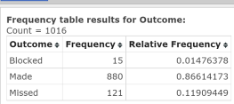
Figure 10. Frequency table for variable outcome that displays frequencies and relative frequencies.
Success is defined here as the outcome in which the attempted field goal is made. Using the existing StatCrunch data file Field Goal Data for the 2013 NFL Season in the Math 216 group folder, you will conduct a test of hypothesis involving the population proportion of NFL field goals made.
Task 9. Use the four-step P‑value approach to test whether the population proportion of NFL field goals made in 2013 exceeds 80% with a level of significance of 5%.
| Step 1. | HO: Population proportion is less than or equal to 0.80. |
| Step 2. | Use StatCrunch to compute the appropriate test statistic and related P‑value. |
Guided Solution 9a
Compute the test statistic P‑value for proportion of NFL field goals made (Step 2).
- Open the StatCrunch data file Field Goal Data for the 2013 NFL Season in the Math 216 groups folder. (For help, see Accessing and Working in StatCrunch on the course home page.)
- Click the menu sequence Stat → Proportion Stats → One Sample → With Data.
- In the Values In box, select the variable Outcome.
- In the Success box, type Made.
- In the Perform section, select Hypothesis test for p.
- In the HO: p box, type 0.80.
In the HA: p box, select > to specify the alternate hypothesis as P.0.80. See Figure 11.
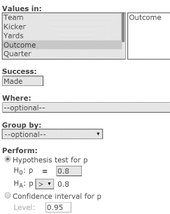
Figure 11. One sample proportion window.
Click Compute to display the Hypothesis test results window, as shown in Figure 12. As the Hypothesis test results window indicates, the test statistic = z = 5.2706288; related P‑value = 0.0001.
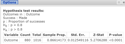
Figure 12. Hypothesis test results window.
| Step 3. | As the P‑value = 0.0001 is less than alpha = 0.05, reject HO. |
| Step 4. | The results support the claim that in 2013 the proportion of attempted NFL field goals that were made exceeded 0.80 or 80%. |
Guided Solution 9b
Copy the Hypothesis test results table into your Word file, ComputerLab4B.
- Type the title: Hypothesis Tests for a Population Proportion-With Sample Data.
- On the next line, copy and paste the Hypothesis test results table you created. (For help with copying StatCrunch data, see Copying Materials from StatCrunch.)
- Save your Word file, ComputerLab4B.
Task 10. Interpretation Question: Hypothesis Test for Population Proportion
Type/paste the four-steps (P‑value approach) to test the hypothesis related to the proportion of 2013 NFL field goals made right under the bottom item in your Word file ComputerLab4B. (If you need help, see the Solution section that follows.)
Remember to save your Word file, ComputerLab4B.
Solution 10
| Step 1. | HO: Population proportion is less than or equal to 0.80. |
| Step 2. | The test statistic = z = 5.2706288; related P‑value = 0.0001. |
| Step 3. | As the P‑value of 0.0001 is less than alpha = 0.05, reject HO. |
| Step 4. | The data supports the claim that 80% of 2013 NFL field goals attempted were made. |
Task 11. Exercise 9 from Elementary Statistics, 6th edition
Exercise 9. Smokers

At a level of significance of 5%, is there enough evidence to support the researcher’s claim?
| Step 1. | HO: Population proportion is greater than or equal to 0.25. |
| Step 2. | Use StatCrunch to compute the appropriate test statistic and related P‑value. |
Guided Solution 11
Use StatCrunch to compute the test statistic and related P‑value that will be used to test the hypothesis (Step 2).
- With a new data table open in StatCrunch, click the menu sequence Stat → Proportion Stats → One Sample → With Summary to display the One Sample Prop. Summary window.
- In the #successes box, type 39 (which is 19.3% × 200 rounded up to 39).
- In the #observations box, type 200.
- In the Perform section:
- Select the Hypothesis test option.
- In the HO: p box, type 0.25.
In the HA: p box, select <. See Figure 13.
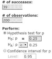
Figure 13. One Sample proportion summary window.
Click Compute to display the Hypothesis test results window, as in Figure 14. As the Hypothesis test results window indicates, the test statistic = z = −1.7962925; related P‑value = 0.0362.

Figure 14. Hypothesis tests results window.
| Step 3. | As the P‑value = 0.0362 is less than alpha = 0.05, reject HO. |
| Step 4. | The sample does support the claim that the proportion of adults who smoke regularly is less than 25%. |
