Mathematics 216 Computer-oriented Approach to Statistics
Computer Lab 5
with Guided Solutions (Technology Manual)
With the aid of the Guided Solutions, use StatCrunch to work through each of the following Activities in your text that relate to Chapter 8 Hypothesis Testing with Two Samples.
We start this Computer Lab with an Equal Variances Test. The content and examples in this computer lab cover all you need to know about this test. Although this is from Chapter 10 of your eText, and not from Chapter 8, you are responsible for it in the computer component of your assignments and exams related to this unit.
Activity 1. Equal Variances Test: Test the Hypothesis that Two Samples Come from Populations that Have Equal Variances
Equal Variances Test
| Step 1. | HO: Variance of Population 1 is equal to Variance of Population 2. |
| Step 2. | Test statistic and related P‑value. |
| Step 3. | Make a decision based on comparing the P‑value with the level of significance, alpha, as follows: |
| Step 4. | State your conclusion. |
Task 1 illustrates the Equal Variances Test.
Task 1. Exercise 19 from Elementary Statistics, 6th edition
Exercise 19. SAT Reading Scores
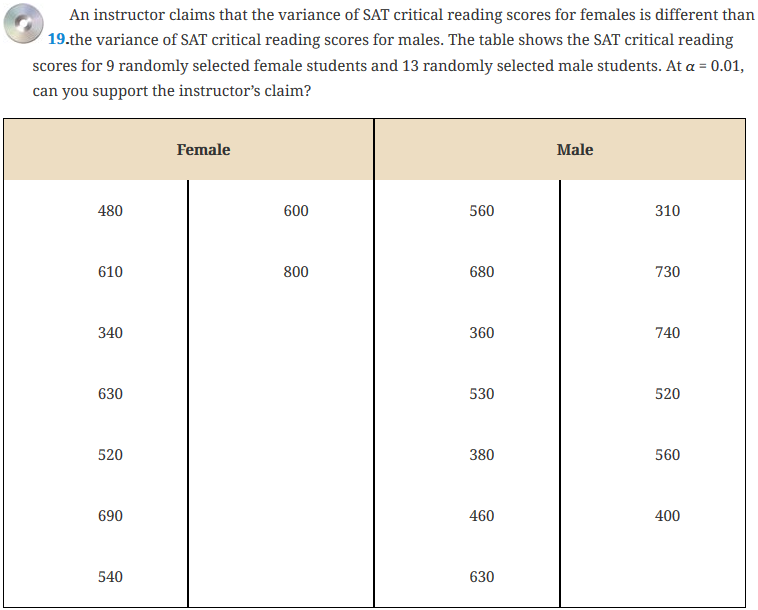
Test the instructor’s claim at a level of significance of 1%. The StatCrunch data file Re10_ex19.txt containing this data is available on StatCrunch stored in the AU Math216 2020 groups folder.
| Step 1. | HO: Variance of Population 1 is equal to Variance of Population 2. |
| Step 2. | Test statistic and related P‑value. |
Guided Solution 1a
StatCrunch will compute an F‑Value test statistic and related P‑value. To determine which set of scores, Female or Male, exhibits the largest variance, use the data file to compute the Variances for the Female and Male SAT Scores.
You will recall that, in computing the F‑Statistic for the Equal Variances Test, the largest sample variance is used in the numerator of the F‑Statistic calculation.
First, use StatCrunch to compute the variances of the Female and Male SAT scores so that you can determine which sample has the largest variance. Next, use StatCrunch to compute the F‑Statistic and its related P‑value, by selecting the sample with the largest variance as the first variable to analyze.
- Open the StatCrunch data file Re10_ex19.txt located in the Math 216 group folder at the StatCrunch website.
- Click the menu sequence Stat → Summary Stats → Columns to display the Summary Stats window.
- Select both the Female and Male variables. (Use the Ctrl key.)
- In the Statistics box, select Variance.
Click Compute to display the variance of both the Female and Male SAT scores. (See Figure 1.) The Male scores exhibit the greatest variance, so Male is the first variable selected in Guided Solution 1b.

Figure 1. Variance of Female and Male SAT scores
Guided Solution 1b
Compute the test statistic and related P‑value (Step 2).
- With the data file Re10_ex19.txt open, click the menu sequence Stat → Variance Stats → Two Sample → With Data to display the Two Sample Variance window.
- Select Male in the Sample 1 box (as Male scores have the greater variance).
- Select Female in the Sample 2 box.
- In the Perform section, select the Hypothesis test option.
In the Perform section, specify the hypotheses:
HO: (Variance 1 squared/Variance 2 squared) = 1.
HA: (Variance 1 squared/Variance 2 squared) not equal to 1. (See Figure 2.)

Figure 2. Two sample variance window.
Click Compute to display the Hypothesis test results window, as in Figure 3. As it indicates, the test statistic = F‑Stat = 1.1672756; related P‑value = 0.8503.
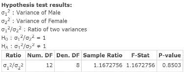
Figure 3. Hypothesis test results window for equal variances test.
| Step 3. | As the P‑value = 0.8503 exceeds alpha = 0.01, do not reject HO. |
| Step 4. | It is reasonable to conclude that the two samples come from populations with equal variances |
Guided Solution 1c
Copy the Hypothesis test results table into a new Word file, ComputerLab5.
- Type the title: Hypothesis Tests with Two Samples.
- On the next line, type the subtitle: Equal Variances Hypothesis Test.
- On the next line, copy and paste the Hypothesis test results table you created. (For help with copying StatCrunch data, see Copying Materials from StatCrunch.)
- Save your Word file, ComputerLab5.
Task 2. Interpretation Question: Equal Variances Test
Type/paste the four-steps (P‑value approach) to test the hypothesis related to Hypothesis test results table below the bottom item in your Word file ComputerLab5. (If you need help, see the Solution section that follows.)
Save your Word file, ComputerLab5.
Solution 2
| Step 1. | Specify the hypotheses: |
| Step 2. | Test statistic and related P‑value: |
| Step 3. | As the P‑value = 0.8503 exceeds alpha = 0.01, do not reject HO. |
| Step 4. | It is reasonable to conclude that the two samples come from populations with equal variances. |
Activity 2. Test hypotheses involving two population means—two independent samples—population standard deviations unknown.
Task 3. Two Population Means Test
Based on the Female and Male SAT reading scores in the data file Re10_ex19.txt, conduct the following test of hypotheses: At a 1% level of significance, test to see if the mean SAT reading scores for the Male students significantly exceeds the mean SAT reading scores for the Female students.
| Step 1. | Specify the hypotheses: HO: μ1 ≤ μ2 or μ1 − μ2 ≤ 0 |
| Step 2. | Use StatCrunch to compute the appropriate test statistic and related P‑value. |
Guided Solution 3a
Compute the test statistic and related P‑value (Step 2).
- With the data file Re10_ex19.txt open, click the menu sequence Stat → T Stats → Two Sample → With Data, to display the Two Sample T Window.
- In the Sample 1 Values box, select Male.
- In the Sample 2 Values box, select Female.
- In the Calculations options box, click the Pool variances box, as in the previous test we found that both samples come from populations of equal variances.
- In the Perform section:
- Select the Hypothesis test option.
Specify the following hypotheses (see Figure 4):
HO: μ1 − μ2 = 0
HA: μ1 − μ2 > 0
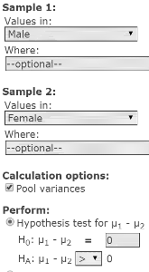
Figure 4. Two Sample T window.
Click Compute to display the Hypothesis test results window, as in Figure 5. As it indicates, the test statistic = T‑Stat = −0.85980103; related P‑value = 0.8.
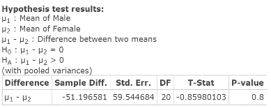
Figure 5. Hypothesis test results window for difference between mean SAT scores.
| Step 3. | As the P‑value = 0.8 exceeds alpha = 0.01, do not reject HO. |
| Step 4. | The sample data does not support the claim that the mean SAT reading scores for males exceeds the mean SAT reading scores for females. |
Guided Solution 3b
Copy the Hypothesis test results table into your Word file, ComputerLab5.
- Type the title: Hypothesis Involving Two Population Means with Population Standard Deviations Unknown.
- On the next line, type: Hypothesis Test Results Table.
- On the next line, copy and paste the Hypothesis test results table you created. (For help with copying StatCrunch data, see Copying Materials from StatCrunch.)
- Save your Word file, ComputerLab5.
Task 4. Interpretation Question: Hypothesis Test for the Population Mean—Population Standard Deviation Unknown
Copy the questions below into your Word file ComputerLab5, below the bottom item.
Type/paste the four-steps (P‑value approach) to follow to test the hypothesis that the mean SAT scores of male students exceeds the mean SAT scores of female students.
Solution:
What two assumptions were made to use the T‑Stat in testing this hypothesis (regarding the SAT scores)?
Solution:
Based on your review of the table, type your answers in the solutions spaces provided. (If you need help answering these questions, see the Solution that follows.) Save your Word file, ComputerLab5.
Solution 4
Four-step P‑value approach:
Question 1.
| Step 1. | Specify the hypotheses: HO: μ1 ≤ μ2 or μ1 − μ2 ≤ 0 |
| Step 2. | Use StatCrunch to compute the appropriate test statistic and related P‑value. |
| Step 3. | As the P‑value = 0.8 exceeds alpha = 0.01, do not reject HO. |
| Step 4. | The sample data does not support the claim that the mean SAT reading scores for males exceeds the mean SAT reading scores for females |
Question 2.
The two assumptions made were:
- Both sample SAT scores come from populations with equal variances.
- As each of the sample sizes is less than 30, you have to test to see if each of the samples, male and female scores, come from a normal population.
Task 5. Review Exercise 19 in Section 10.3: Test assumptions made.
In using the T‑Stat to conduct the hypothesis test to see if mean SAT reading scores for males exceed that of females, two assumptions were made. Use StatCrunch to test the two assumptions made:
- Equal Variances Assumption
Using the T‑Stat to conduct the test that compares the mean SAT reading scores assumes that the sample of male SAT scores and the sample of female SAT scores both come from populations with equal variances. This assumption was made as we clicked on the pool variances option under Calculator options, when computing the test statistic = −0.85980103 and related P‑value = 0.80. You will recall that in a previous exercise we found that it is reasonable to assume that the two samples of SAT scores come from populations with equal variances. - Normality Assumption
Using the T‑Stat to conduct the test that compares the mean SAT reading scores assumes that the sample SAT scores both come from normal populations.
We will now apply the Shapiro-Wilk Test to each of the two samples of SAT scores.
| Step 1. | Specify the hypotheses: HO: The population is normally distributed. |
| Step 2. | Use StatCrunch to compute the Shapiro-Wilk test statistic and related P‑value for both the male and female samples of SAT scores. |
Guided Solution 5
Use StatCrunch to Compute the Shapiro-Wilk test statistic and P‑value (Step 2).
- With the data file Re10_ex19.txt open, click the menu sequence Stat → Goodness-of-fit → Normality Test.
- In the Select columns box, select both variables, Female and Male (use the Ctrl key).
- In the Test box, select Shapiro-Wilk.
Click Compute to display the Hypothesis test results window, as shown in Figure 6. For the Female sample, the test statistic = .98432047; P‑value = 0.9828. For the Male sample, the test statistic = .9527315; P‑value = 0.6402.

Figure 6. Shapiro-Wilk results window.
| Step 3. | For both samples, the P‑value exceeds alpha, so we do not reject HO for each sample tested. |
| Step 4. | It is reasonable to assume that both samples come from normal populations. As a result, we can feel confident in the conclusion that the sample data does not support the claim that the mean SAT reading scores for males exceeds the mean SAT reading scores for females. |
Task 6. Exercise 19 from Elementary Statistics, 6th edition
Exercise 19. Tensile Strength
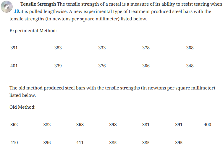
At a 1% level of significance, test to see if there is a difference in mean tensile strengths between the new experimental treatment and the old treatment. Assume that both samples of tensile strengths come from populations with equal variances. Use the four-step P‑value approach.
Data on the both the new and the old experimental treatment types are in the StatCrunch data file Ex8_2-19.txt, which is available in the Math 216 group folder.
| Step 1. | Specify the hypotheses: HO: μ1 = μ2 or μ1 − μ2 = 0 |
| Step 2. | Use StatCrunch to compute the appropriate test statistic and related P‑value. |
Guided Solution 6a
Compute the test statistic and related P‑value:
- To conduct a test of hypothesis comparing the mean tensile strengths, you must open the StatCrunch data file Ex8_2-19.txt. (For help, see Accessing and Working in StatCrunch on the course home page.)
- Click the menu sequence Stat → T‑Stats → Two Sample → With Data, to open the Two Sample T window.
- In the Sample 1 Values box, select New method.
- In the Sample 2 Values box, select Old method.
- In the Calculations options box, click the Pool variances box (as the question assumes equal population variances).
- In the Perform section:
- Select the Hypothesis test option.
Specify the hypotheses:
HO: μ1 − μ2 = 0
HA: μ1 − μ2 ≠ 0
Click Compute to display the Hypothesis test results window, as in Figure 7. As it indicates, the test statistic = T‑Stat = −2.7649555; related P‑value = 0.0116.
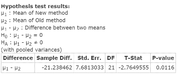
Figure 7. Hypothesis test results window for difference between mean tensile strengths.
| Step 3. | As the P‑value = 0.0116 exceeds alpha = 0.01, do not reject HO. |
| Step 4. | The sample data does not support the claim that there is a significant difference in mean tensile strengths between the New and Old methods. |
Guided Solution 6b
Copy the Hypothesis test results table into your Word file, ComputerLab5.
- Type the title: Hypothesis Involving Two Population Means with Population Standard Deviations Unknown.
- On the next line, type: Exercise 19 Section 8.2.
- On the next line, copy and paste the Hypothesis test results table you created. For help with copying StatCrunch data, see Copying Materials from StatCrunch.
- Save your Word file, ComputerLab5.
Task 7. Interpretation Question: Hypothesis Test for the Population Mean—Population Standard Deviation Unknown
Copy the question below into your Word file ComputerLab5, below the bottom item.
In using the T‑Stat to test the mean tensile strengths produced under the New vs. Old methods in Exercise 19 Section 8.2, what two assumptions were made?
Solution:
Based on your review of the table, type your answer in the solution space provided. (If you need help answering the question, see the Solution that follows.) Save your Word file, ComputerLab5.
Solution 7
Two assumptions made were:
- The two sample tensile come from populations with equal variances.
- As each of the sample sizes is less than 30, you must test to see if each of the samples, New method and Old method, come from normal populations.
Task 8. Exercise 19 from Section 8.2 of your eText: Equal Variances Test
In using the T‑Stat to conduct the hypothesis test comparing mean tensile strengths, it was assumed that both samples come from populations with equal variances (as the pooled variance was used in computing the T‑Stat). Use StatCrunch to test this assumption at a 1% level of significance.
Test the Equal Variances Assumption: Four-step P‑value Approach.
| Step 1. | HO: Variance of Population 1 is equal to Variance of Population 2. |
| Step 2. | Test statistic and related P‑value. |
Guided Solution 8a
Compute the variances for the new method and old method tensile strengths.
StatCrunch will compute an F‑Value test statistic and related P‑value. To compute the test statistic and related P‑value you must open the StatCrunch data file and determine which set of scores, New method or old Method, exhibits the largest variance.
You will recall that when computing the F‑Statistic for the Equal Variances Test, the largest sample variance should be used in the numerator of the F‑Statistic calculation. This will be the sample selected as the first variable to analyze in the T‑Test. This means that we have to use Minitab to compute the variance of each sample as follows.
- Open the data file Ex8_2-19.txt. (For help, see Accessing and Working in StatCrunch on the course home page.)
- Click the menu sequence Stat → Summary Stats → Columns, to open a Summary Stats window.
- In the Select columns box, select both the New method and Old method variables. (Use the Ctrl key.)
- In the Statistics box, select Variance.
Click Compute to display the variance of both samples, as in Figure 8. The New method tensile strengths exhibit the greatest variance, so New method will be the first variable selected in Guided Solution 8b.

Figure 8. Variance of tensile strengths for each of the two samples2019
Guided Solution 8b
Computing the test statistic and related P‑value: Equal Variances Test
- With the data file Ex8_2-19.txt open, click the menu sequence Stat → Variance Stats → Two Sample → With Data, to display the Two Sample Variance window.
In the Sample 1 box, select New method (as this sample has the greater variance). In the Sample 2 box, select Old method.
- In the Perform section:
- Select the Hypothesis test option.
Specify the hypotheses:
HO: (Variance 1 squared/ Variance 2 squared) = 1.
HA: (Variance 1 squared/ Variance 2 squared) does not equal 1.
Click Compute to display the Hypothesis test results window, as in Figure 9. The test statistic = F‑Stat = 2.3615308; related P‑value = 0.1668.
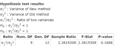
Figure 9. Hypothesis test results window for equal variances test.
| Step 3. | As the P‑value = 0.1668 exceeds alpha = 0.01, do not reject HO. |
| Step 4. | It is reasonable to conclude that each of the two samples come from populations with equal variances, at a 1% level of significance. |
Task 9. Exercise 19 Tensile Strength, in Section 8.2 of your eText: Normality Test
In using the T‑Stat to conduct the hypothesis test comparing mean tensile strengths, it was assumed that both samples come from normal populations. Use StatCrunch to test this assumption.
| Step 1. | For each sample of tensile strengths: |
| Step 2. | Use StatCrunch to compute the Shapiro-Wilk test statistic and related P‑value for each of the two samples. |
Guided Solution 9
Apply the Shapiro-Wilk Test to each of the two samples of tensile strengths (Step 2). Use StatCrunch to compute the Shapiro-Wilk test statistic and P‑value.
- With the data file Ex8_2-19.txt open, click the menu sequence Stat → Goodness-of-fit → Normality Test.
- In the Select columns box, select both variables: New method, and Old method. (Use the Ctrl key.)
- In the Test box, select Shapiro-Wilk.
Click Computeto display theHypothesis test results window, as in Figure 10. For the New method sample the test statistic = .95600674; P‑value = 0.7396. For the Old method sample, the test statistic = .96124619; P‑value = 0.7728.

Figure 10. Shapiro-Wilk results window
| Step 3. | For both samples, the P‑value exceeds alpha so we do not reject HO for each sample tested. |
| Step 4. | It is reasonable to assume that both samples come from normal populations. As a result, we can feel confident in the conclusion that there is no significant difference in the mean tensile strength produced by the New method vs. the Old method. |
Activity 3. Test hypotheses involving two population means—two dependent samples—population standard deviation unknown
Task 10. Exercise 13 from Elementary Statistics, 6th edition
Exercise 13. Headaches
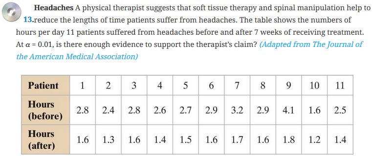
At the level of significance of 5%, test to see if there is enough evidence to support the therapist’s claim. The StatCrunch data file Ex8_3-13.txt, in the eText data folder, shows the number of hours per day 11 patients suffered from headaches before and after 7 weeks of receiving the physical therapy treatment.
| Step 1. | Let d = (Patient headache time before treatment − Patient headache time after treatment) = (Before − After). |
| Step 2. | Use StatCrunch to compute the appropriate test statistic and related P‑value. |
Guided Solution 10a
Compute the test statistic and related P‑value.
- Open the StatCrunch data file Ex8_3-13.txt located in the AU Math 216 group folder at the StatCrunch website.
- Click the menu sequence Stat → T‑Stats → Paired, to display the Paired T window.
- In the Sample 1 box, select Before (as Before comes first in calculating d).
- Click the Save differences option to create a column of differences.
- In the Sample 2 box, select After.
- In the Perform section:
- Select the Hypothesis test option.
Specify the hypotheses:
HO: μD = 0
HA: μD > 0
Click Compute to display the Hypothesis test results window, as in Figure 11. As it indicates, the test statistic = T‑Stat = 9.4290807; related P‑value = 0.0001.

Figure 11. Hypothesis test results window for difference between headache times.
| Step 3. | As the P‑value = 0.0001 is less than alpha = 0.05, reject HO. |
| Step 4. | The sample data does support the therapist’s claim that the therapy treatment has significantly reduced patient headache time. |
Guided Solution 10b
Copy the Hypothesis test results table into your Word file, ComputerLab5.
- Type the title: Hypothesis Involving Two Population Means with Dependent Samples—Population Standard Deviation Unknown.
- On the next line, type the subtitle: Exercise 13 Section 8.3.
- On the next line, copy and paste the Hypothesis test results table you created. (For help with copying StatCrunch data, see Copying Materials from StatCrunch.)
- Save your Word file, ComputerLab5.
Task 11. Interpretation Question: Hypothesis Test for the Population Mean—Dependent Samples—Population Standard Deviation Unknown. Assumptions Made
Copy the question below into your Word file ComputerLab5, under the bottom item.
What key assumption was made when you tested the therapist’s claim that the treatment reduced patient headache time per day?
Solution:
Based on your review of the pasted table, type your answer in the solution space provided. (If you need help answering the question, see the Solution that follows.) Save your Word file, ComputerLab5.
Solution 11
- It was assumed that the sample of differences, d, comes from a normal population. As the sample of differences d = (Before − After) is less than 30 (only 11 differences) you will have to conduct a normality test on the sample of 11 differences, which should now be displayed in the 3rd column of the data table “Differences”?
Task 12. Exercise 13 Headaches, from Section 8.3 of your eText: Normality Test
In using the T‑Stat to conduct the hypothesis test regarding physical therapy treatment and patient headache time, it was assumed that d, the sample of differences, comes from a normal population. Use StatCrunch to test this assumption at the 5% level of significance. Apply the Shapiro-Wilk test to the sample of differences.
| Step 1. | HO: The population of differences is normally distributed. |
| Step 2. | Use StatCrunch to compute the Shapiro-Wilk test statistic and related P‑value for the sample of differences, which is displayed in the data table column Differences. |
Guided Solution 12
Using StatCrunch to Compute the Shapiro-Wilk test statistic and P‑value
- With the data file Ex8_3-13.txt open, click the menu sequence Stat → Goodness-of-fit → Normality Test.
- In the Select columns box, select the variable Differences.
- In the Test box, select Shapiro-Wilk.
Click Compute to display the Hypothesis test results window, as shown in Figure 12. For d, the column of Differences, the test statistic = 0.8103566; P‑value = 0.0129.

Figure 12. Shapiro-Wilk results window applied to column of differences.
| Step 3. | As the P‑value is less than alpha of 5%, reject HO for the sample of differences. |
| Step 4. | The sample of differences used in testing the therapists claim does not come from a normal population. As a result, you cannot use the T‑Stat in testing the effectiveness of the therapist’s treatment in reducing patient headache time. You cannot make any valid statistical conclusion using the sample of 11 differences to test the therapist’s claim regarding the effectiveness of the therapy treatment. One alternative is to randomly collect another 19 pairs of before and after data, to make the total sample size at least 30 paired differences. You could then use the T‑Stat in testing the effectiveness of the therapist’s treatment. |
Task 13. Exercise 10 from Elementary Statistics, 6th edition
Exercise 10. SAT Scores
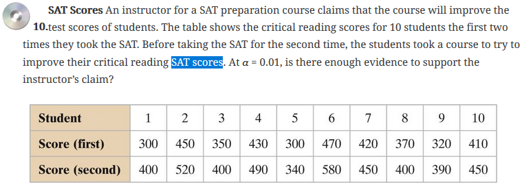
At the level of significance of 1%, test to see if there is enough evidence to support the instructor’s claim? The data are contained in the StatCrunch data file Ex8_3-10.txt, which is available in the Math 216 groups folder.
| Step 1. | Let d = (First Score – Second Score). |
| Step 2. | Use StatCrunch to compute the appropriate test statistic and related P‑value. |
Guided Solution 13
Use StatCrunch to compute the test statistic and related P‑value that will be used to test the hypothesis (Step 2). As the population standard deviation is unknown, you will use the t statistic in this test.
- Open the StatCrunch data file Ex8_3-10.txt. (For help, see Accessing and Working in StatCrunch on the course home page.)
- With the data file Ex8_3-13.txt open, click the menu sequence Stat → T‑Stats → Paired, to open the Paired T window.
- In the Sample 1 box, select First score (as it comes first in the calculation of d).
- in the Sample 2 box, select Second score.
- Click Save differences to create a column of differences.
- In the Perform section:
- Select the Hypothesis test option.
Specify the hypotheses:
HO: μD = 0
HA: μD < 0
Click Compute to display the Hypothesis test results window, as in Figure 13. The test statistic = T‑Stat = −6.8033605 Related P‑value = 0.0001

Figure 13. Hypothesis test results window for SAT score differences.
| Step 3. | As the P‑value = 0.0001 is less than alpha = 0.01, reject HO. |
| Step 4. | The sample data does support the instructor’s claim that the preparation test improves SAT critical reading scores. |
Task 14. Exercise 10 from Section 8.3 of your eText: Normality Test
In using the T‑Stat in the test of hypothesis, you assumed that d, the sample of differences, comes from a normal population. As the sample size is only 10 paired differences, you must now apply the Shapiro-Wilk Test to the sample of differences to test for normality.
Use StatCrunch to test this assumption at the 1% level of significance.
| Step 1. | HO: The population of differences is normally distributed. |
| Step 2. | Use StatCrunch to compute the Shapiro-Wilk test statistic and related P‑value for the sample of differences. |
Guided Solution 14
Use StatCrunch to compute the Shapiro-Wilk test statistic and P‑value (Step 2).
- With the data file Ex8_3-10.txt open, click the menu sequence Stat → Goodness-of-fit → Normality Test.
- In the Select columns box, select the variable Differences.
- In the Test box, select Shapiro-Wilk.
Click Compute to display the Hypothesis test results window, as shown in Figure 14. For d, the column of Differences, the test statistic = 0.90153406; P‑value = 0.2277.

Figure 14. Shapiro-Wilk results window applied to column of differences.
| Step 3. | As the P‑value is greater than alpha of 1%, do not reject HO for the sample of differences. |
| Step 4. | It is reasonable to conclude that the sample of differences in SAT scores does come from a normal population. You can now have confidence in the conclusion made when using the T‑Stat to support the instructor’s claim regarding the effectiveness of the SAT preparation test; that is, it appears that the preparation test did improve SAT critical reading scores. |
Activity 4. Test Hypotheses Involving Two Population Proportions
Task 15. Exercise 9 from Elementary Statistics, 6th edition
Exercise 9.

At the level of significance of 5%, test to see if there is enough evidence to support the claim that the proportion of males enrolled in college is significantly less than the proportion of females enrolled in college.
| Step 1. | Let p1 = Population proportion of males enrolling in college. HO: p1 − p2 ≥ 0 |
| Step 2. | Use StatCrunch to compute the appropriate test statistic and related P‑value. |
Guided Solution 15a
Computing the test statistic and related P‑value (Step 2).
- Open a new data table in StatCrunch.
- Click the menu sequence Stat → Proportion Stats → Two Sample → With Summary, to display a Two Sample Prop Summary window.
- In the Sample 1 section:
- In the # successes box, type 78 (39% × 200 = 78).
- In the # observations box, type 200.
- In the Sample 2 section:
- In the # successes box, type 99 (45% × 220 = 99).
- In the # observations box, type 220.
- In the Perform section:
- Select the Hypothesis test option.
Specify the hypotheses:
HO: p1 − p2 = 0
HA: p1 − p2 < 0
-
Click Compute to display the Hypothesis test results window, as in Figure 15. The test statistic = Z‑Stat = −1.2436909; related P‑value = 0.1068.

Figure 15. Hypothesis test results window for difference in proportion
| Step 3. | As the P‑value 0.1068 is greater than alpha = 0.05, do not reject HO. |
| Step 4. | The sample data does not support the claim that the proportion of males enrolling in college is significantly less than the proportion of females enrolling in college. |
Guided Solution 15b
Copy the Hypothesis test results table into your Word file, ComputerLab5.
- Type the title: Hypothesis Test Involving Two Population Proportions With Summary Data
- On the next line, type the subtitle: Exercise 9 Section 8.4.
- On the next line, copy and paste the Hypothesis test results table you created. For help with copying StatCrunch data, see Copying Materials from StatCrunch.
- Save your Word file, ComputerLab5.
Task 16. Interpretation Question: Hypothesis Test Involving Two Population Proportions With Summary Data
In your ComputerLab5 Word file, below the bottom item, type/paste the four-steps (P‑value approach) to test the hypothesis that the proportion of males enrolled in college is less than the proportion of females enrolled in college. (If you need help answering the question, see the Solution that follows.) Save your Word file, ComputerLab5.
Solution 16
- four-step P‑value Approach
| Step 1. | Specify the hypotheses: HO: p1 − p2 ≥ 0 |
| Step 2. | Use StatCrunch to compute the appropriate test statistic and related P‑value. The test statistic = Z‑Stat = −1.2436909 Related P‑value = 0.1068. |
| Step 3. | As the P‑value 0.1068 is greater than alpha = 0.05, do not reject HO. |
| Step 4. | The sample data does not support the claim that the proportion of males enrolling in college is significantly less than the proportion of females enrolling in college. |
Task 17. College Giving: Two Population Proportions Test
Here, we will conduct another hypothesis test involving two population proportions. Figure 16 describes a survey questionnaire that was completed by all 210 staff of a small college. The survey responses have been entered into the StatCrunch data file College_Giving, which is in the Math 216 groups folder.
| Please check the survey codes that apply to you below. | Variable | Text Code |
| 1. Please check your gender. | Gender | |
| ☐ male | ______ M | |
| ☐ female | ______ F | |
| 2. Have you have engaged in volunteer activity this year? | Volunteer | |
| ☐ yes | _______Y | |
| ☐ no | _______N |
Figure 16. Volunteer questionnaire.
Using the survey responses data file College_Giving, conduct a hypothesis test to see if there is enough evidence to support the claim that the proportion of females engaged in volunteer activity in the current year is significantly greater than the proportion of males engaged in volunteer activity. Test at the 1% level of significance.
| Step 1. | Let p1 = population proportion of females engaged in volunteer activity. HO: p1 − p2 ≤ 0 |
| Step 2. | Use StatCrunch to compute the appropriate test statistic and related P‑value. |
Guided Solution 17
Compute the test statistic and related P‑value. (Step 2)
- Open the StatCrunch data file College_Giving.txt. (For help, see Accessing and Working in StatCrunch on the course home page.)
- Click the menu sequence Stat → Proportion Stats → Two Sample → With Data, to display the Two Sample Proportions window.
- In the Sample 1 section:
- In the Values box, select Volunteer.
- In the Success box, type Y.
- In the Where box, type: Gender = F
- In the Sample 2 section:
- In the Values box, select Volunteer.
- In the Success box, type Y.
- In the Where box, type: Gender = M
- In the Perform section:
- Select the Hypothesis test option.
Specify the hypotheses:
HO: p1 − p2 = 0
HA: p1 − p2 > 0
Click Compute to display the Hypothesis test results window, as in Figure 17. The test statistic = Z‑Stat = 13.247604; related P‑value < 0.0001.

Figure 17. Hypothesis test results window for difference in proportion
| Step 3. | As the P‑value 0.0001 is less than alpha = 0.01, reject HO. |
| Step 4. | The sample data does support the claim that the proportion of females engaged in volunteer activity is significantly greater than the proportion of males engaged in volunteer activity. |
